From Pretrained Model to Deployed Assistant

Alignment, Decoding, and Distillation

Robert Minneker

2026-02-12

Sources

Content derived from: J&M Ch. 8 (Transformers), Ch. 7 (Large Language Models)

Administrivia

• Project checkpoints due Today!

Learning Objectives

By the end of this lecture, you will be able to:

1. Explain the difference between training-time, inference-time, and deployment-time control in LLMs

2. Implement and compare decoding algorithms

3. Describe how alignment (SFT, RLHF, DPO) modifies model behavior

4. Explain how distillation enables efficient deployment

• Bold items are directly assessed in Assignment 3
• Items 1-2 prepare for Part 1 (implementing attention)
• Items 2-3 prepare for Part 2 (decoding algorithms)
• Item 3 prepares for the knowledge distillation bonus

Today’s roadmap

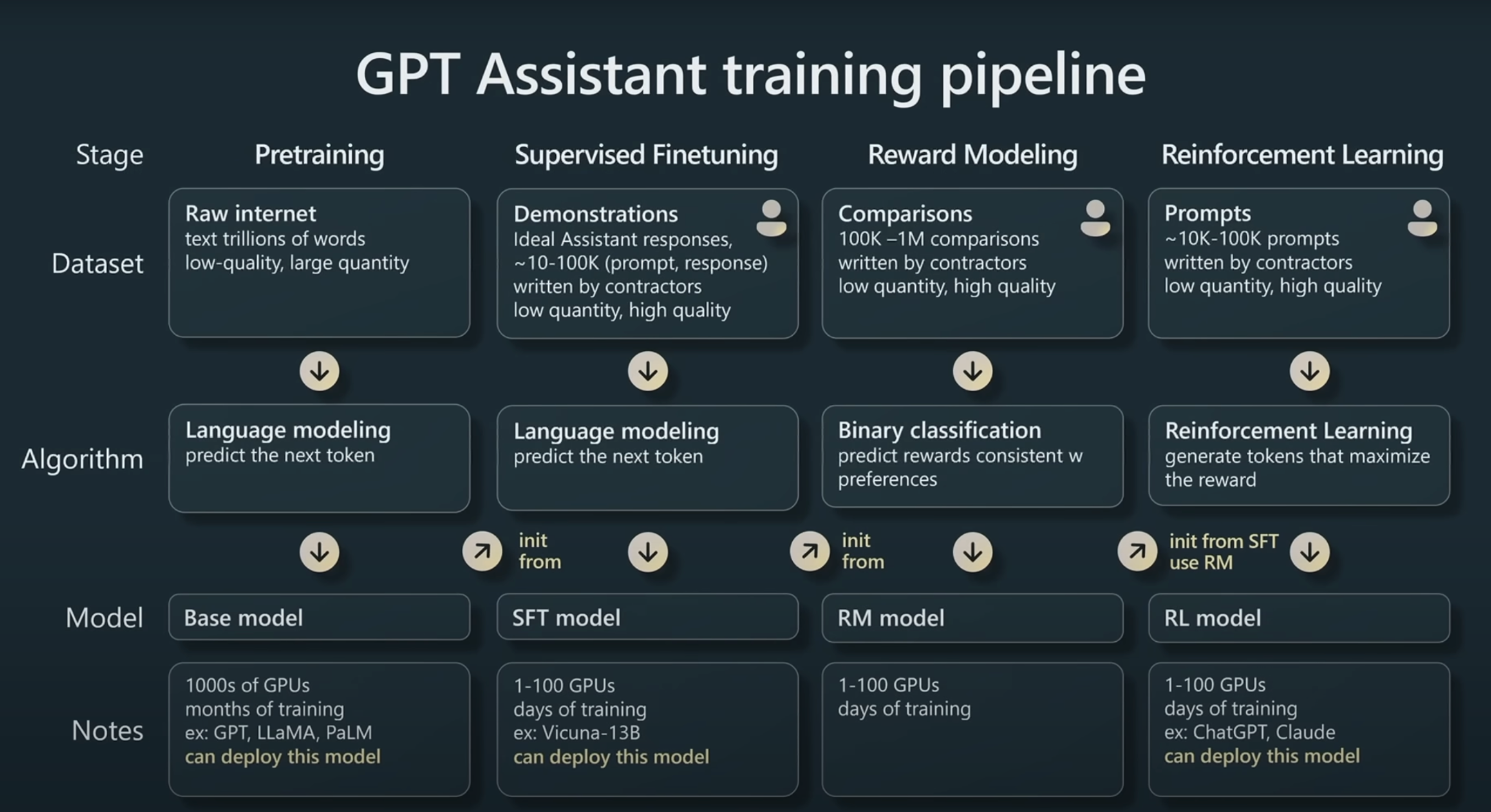
Karpathy (2023): GPT Assistant Training Pipeline

Last time: Pretraining (Stage 1). Today: everything after.

• Part 5: Instruction Tuning (SFT) — teaching the model to follow instructions
• Part 6: RLHF & DPO — aligning with human preferences
• Part 7: Decoding Algorithms — how LLMs actually generate text
• Part 8: Knowledge Distillation — deploying smaller models

• This image from Karpathy’s “State of GPT” talk shows the full training pipeline
• We covered pretraining last lecture
• Today covers everything that happens after pretraining to produce a useful assistant

Part 5: Instruction Tuning

Base models complete text — they don’t follow instructions

Base Model

Prompt: "Summarize this article: The economy grew..."

"...by 3.2% in the third quarter, beating analyst expectations. Experts say this trend is likely to continue..."

Continues the article instead of summarizing

Instruction-Tuned Model

Prompt: "Summarize this article: The economy grew..."

"The article reports that the economy expanded by 3.2% in Q3, exceeding expectations due to strong consumer spending."

Actually summarizes as instructed

• Base models are trained to predict what comes next in web text
• Instructions like “summarize” are rare in training data
• The model has the capability—it just needs to learn to apply it

Supervised Fine-Tuning (SFT) on instruction-response pairs

Training data format:

Instruction: Translate "Hello, how are you?" to French.

Response: "Bonjour, comment allez-vous?"

SFT objective:

\[ \mathcal{L}_{\text{SFT}} = -\sum_{i=1}^{N} \log P_\theta(y_i \mid x_i) \]

• \(x_i\): instruction (input)
• \(y_i\): desired response (output)
• Same cross-entropy loss, but on curated instruction data

• SFT is standard supervised learning on instruction-response pairs
• The model already has capabilities from pretraining
• SFT teaches it to activate those capabilities on command

Instruction tuning: Implementation details

Formatting data for instruction-tuned models:

# For summarization with instruction-tuned models
def prepare_for_summarization(article, tokenizer):
    prompt = f"Summarize the following article.\n\n{article}\n\nTL;DR:"
    return tokenizer(prompt, return_tensors="pt")

# System prompts set the model's "persona"
system_prompt = "You are a helpful assistant and an expert at summarizing articles."

Fine-tuning with label masking (for training summarization models):

# We only want to train on generating the SUMMARY, not the article
labels = input_ids.clone()
labels[:prompt_length] = -100  # -100 is ignored by CrossEntropyLoss

# The model learns: given article, predict summary tokens

• These details are directly relevant for Assignment 3 knowledge distillation
• The -100 trick lets us train on partial sequences
• System prompts are how we configure model behavior

Large models are expensive to deploy

70B+

parameters in frontier models

$$$

GPU costs for serving

High latency

slow responses at scale

We want similar quality at lower cost.

Preview: Knowledge Distillation (Part 8)

We can train a smaller “student” model to mimic the large model’s behavior — getting most of the quality at a fraction of the cost.

Before turning to efficiency, we’ll address a deeper limitation of SFT: It only learns from one correct answer per instruction. Can we do better?

• This creates a natural bridge: SFT works → but it’s expensive (Part 8) → and it has limitations (RLHF)
• Distillation is about deployment efficiency, not improving alignment
• The “one correct answer” limitation motivates RLHF in Part 6

Part 6: Preference Alignment with RLHF

Why RLHF? SFT isn’t enough

SFT limitations:

• One "correct" answer per instruction
• Can't encode preferences between valid responses
• Expensive to write high-quality responses
• May learn to imitate surface patterns

RLHF advantages:

• Captures human preferences between options
• Easier to judge than to write
• Learns subtle quality distinctions
• Optimizes for what humans actually want

Key insight: It’s easier to say “A is better than B” than to write the perfect A.

• This is the insight that enabled ChatGPT’s success
• Humans are better at comparison than absolute quality judgments
• RLHF leverages this comparative ability

RLHF: The three-step process

1

Collect Preference Data

For each prompt, generate multiple responses. Humans rank: A > B or B > A

↓

2

Train Reward Model

Learn to predict human preferences: r(x, y) → scalar score

↓

3

Optimize LLM with RL

Use PPO to maximize expected reward while staying close to SFT model

• Each step builds on the previous
• The reward model acts as a proxy for human judgment
• RL optimizes the LLM to generate high-reward responses

RLHF data flow

%%{init: {"theme":"base","themeVariables":{"fontFamily":"Inter, system-ui, sans-serif","fontSize":"16px","primaryColor":"#eef2f7","primaryTextColor":"#0f172a","lineColor":"#475569","tertiaryColor":"#e2e8f0"},"flowchart":{"curve":"basis","nodeSpacing":30,"rankSpacing":50}}}%%
flowchart LR
    P["Prompts"] --> M["SFT Model πθ"]
    M --> RA["Response A"]
    M --> RB["Response B"]
    RA --> H["Human Rater"]
    RB --> H
    H -->|"A ≻ B"| RM["Reward Model rθ"]
    RM -->|"r(x,y)"| PPO["PPO"]
    PPO -->|"Update πθ"| M

The reward model is a learned proxy for human judgment — it scores responses so we don’t need a human in the loop at training time.

• The flow diagram shows how data moves through the RLHF pipeline
• Prompts go to the SFT model, which generates multiple responses
• Humans compare pairs — this is cheaper than writing ideal responses
• The reward model learns from these comparisons
• PPO uses the reward model to update the policy, with a KL penalty to stay close to the SFT model

Reward model intuition: Learning from comparisons

Prompt: "Explain gravity to a 5-year-old"

Response A ✓ preferred
"Gravity is like an invisible magnet in the Earth that pulls everything down — that's why when you jump, you come back!"

Response B
"Gravity is a fundamental force described by general relativity as the curvature of spacetime caused by mass-energy..."

Reward model assigns scores: r(A) = 2.4, r(B) = 0.8
P(A ≻ B) = σ(2.4 − 0.8) = σ(1.6) ≈ 0.83

This intuition leads to the Bradley-Terry model →

• Human annotators compare pairs of responses — they don’t assign absolute scores
• The reward model learns to produce scalar scores consistent with pairwise preferences
• The sigmoid of the score difference gives the probability that A is preferred over B

Training the reward model

Bradley-Terry preference model:

\[ P(A \succ B) = \sigma(r_\theta(x, y_A) - r_\theta(x, y_B)) \]

Reward model loss:

\[ \mathcal{L}_{\text{RM}} = -\mathbb{E}_{(x, y_w, y_l)} \left[ \log \sigma(r_\theta(x, y_w) - r_\theta(x, y_l)) \right] \]

• \(y_w\): preferred (winning) response
• \(y_l\): dispreferred (losing) response
• \(\sigma\): sigmoid function

The reward model learns to assign higher scores to preferred responses.

• This is basically binary classification: which response is better?
• The reward model is typically a transformer initialized from the LLM
• It outputs a single scalar for each (prompt, response) pair

Optimizing the LLM with reinforcement learning

Objective:

\[ \max_\theta \mathbb{E}_{y \sim \pi_\theta(y|x)} [r(x, y)] - \beta \cdot \text{KL}[\pi_\theta \| \pi_{\text{ref}}] \]

Reward Maximization

E[r(x, y)]

Generate responses that score high

KL Penalty

-β · KL[π || π_ref]

Don't deviate too far from SFT model

• PPO (Proximal Policy Optimization) is commonly used
• KL penalty prevents “reward hacking”

• Without KL penalty, the model might exploit reward model weaknesses
• β controls the trade-off between reward and staying close to SFT
• This is why it’s called “alignment”—aligning LLM with human preferences

From RLHF to DPO: What changes?

RLHF

• Train a separate reward model
• Run PPO optimization loop
• Complex, unstable training
• Three separate stages

→

DPO

• No reward model needed
• No RL loop required
• Directly optimize preference pairs
• Standard supervised learning

Key insight: Same preference data, dramatically simpler training.

• DPO achieves similar results to RLHF with much less engineering complexity
• The next slide shows how this works mathematically
• No equations on this slide — the intuition is what matters

Alternatives to RLHF: Direct Preference Optimization

Key insight: The optimal RLHF policy has a closed-form relationship with the reward model. DPO exploits this to optimize directly on preference pairs — no reward model or RL needed.

DPO loss (Rafailov et al., 2023):

\[ \mathcal{L}_{\text{DPO}} = -\mathbb{E}\left[\log \sigma\left(\beta \log \frac{\pi_\theta(y_w|x)}{\pi_{\text{ref}}(y_w|x)} - \beta \log \frac{\pi_\theta(y_l|x)}{\pi_{\text{ref}}(y_l|x)}\right)\right] \]

Reading the formula: increase the probability of the preferred response \(y_w\) (relative to the reference model) and decrease the probability of the dispreferred response \(y_l\).

RLHF

Preferences → Reward Model → RL

Complex, unstable, expensive

DPO

Preferences → Direct optimization

Simpler, stable, supervised learning

• DPO reformulates RLHF as a classification problem
• The log-ratio terms measure how much the model’s preferences have shifted from the reference
• No need to train a separate reward model — increasingly popular due to simplicity

Alignment goals: Helpful, Harmless, Honest

Helpful

Answers questions effectively
Completes requested tasks
Provides useful information

Harmless

Refuses dangerous requests
Avoids harmful content
Doesn't assist malicious use

Honest

Acknowledges uncertainty
Doesn't make things up
Corrects mistakes

Tension

These goals can conflict: A helpful answer to a harmful request is itself harmful.

• This “HHH” framework guides alignment research
• Balancing these goals is challenging
• Perfect alignment remains an open problem

Concept check

Quick questions (think for 30 seconds):

1. In the RL objective, what happens if we set β = 0?
2. An RLHF-trained chatbot starts adding “As an AI language model…” to every response. What went wrong?

RL Objective reminder: \[ \max_\theta \mathbb{E}_{y \sim \pi_\theta(y|x)} [r(x, y)] - \beta \cdot \text{KL}[\pi_\theta \| \pi_{\text{ref}}] \]

• β = 0: No KL penalty → model only maximizes reward → reward hacking (learns to exploit quirks in the reward model rather than being genuinely helpful)
• β → ∞ (bonus): Model stays identical to the SFT model — no alignment improvement
• The repetitive disclaimer suggests the reward model learned that “safe-sounding” responses always get high human preference scores, so the model overfit to adding disclaimers
• Both are examples of alignment being hard: optimizing a proxy (reward model) isn’t the same as optimizing true helpfulness
• Give students 30–60 seconds to think, then discuss

From training to generation

We’ve covered how LLMs are trained to be helpful:

1. Pretraining — learn language from raw text
2. SFT — learn to follow instructions (Part 5)
3. RLHF/DPO — align with human preferences (Part 6)

Now: how do they actually generate text?

Given a trained model and a prompt, how do we produce an output — one token at a time?

But note: what you put in matters as much as how tokens come out. We’ll cover the output side today (decoding), and the input side next time (prompting, in-context learning, reasoning).

• This is the training → inference boundary
• Everything so far was about making the model good
• Now we ask: given a good model, how do we use it?
• Two sides of the coin: how you prompt (input) and how you decode (output)
• Today covers decoding; next lecture covers prompting and reasoning strategies

Three control knobs in LLM systems

Training-time

(change weights)

• SFT
• RLHF
• DPO

Inference-time

(change decoding)

• Greedy
• Temperature
• Top-k / Top-p

Deployment-time

(change size)

• Knowledge distillation

These mechanisms operate on different axes but interact in final behavior.

• This is the big picture: three independent axes for controlling LLM behavior
• Training-time changes what the model knows and values
• Inference-time changes how tokens are selected from the distribution
• Deployment-time changes the model’s size and efficiency

Training vs. inference: Different levers

Training (shapes probabilities)

• Alignment modifies the token distribution
• Changes relative likelihoods

Inference (selects from distribution)

• Decoding determines which tokens get chosen

These interact in practice:

• Greedy decoding can amplify repetitive artifacts from training
• High temperature increases hallucination risk regardless of alignment
• Beam search often reduces diversity even in well-aligned models

• This is the bridge between Part 6 (alignment) and Part 7 (decoding)
• Training makes certain tokens more likely, but decoding decides what actually gets output
• Understanding both is necessary to understand LLM behavior in practice

Part 7: Text Generation and Decoding

The autoregressive generation loop

def generate(model, prompt_ids, max_new_tokens=50):
    input_ids = prompt_ids

    for _ in range(max_new_tokens):
        # Forward pass: get logits for all positions
        logits = model(input_ids)  # (B, seq_len, vocab_size)

        # Extract logits for the LAST position only
        next_token_logits = logits[:, -1, :]  # (B, vocab_size)

        # DECODE: Select next token (this is where methods differ!)
        next_token = decode(next_token_logits)

        # Append and continue
        input_ids = torch.cat([input_ids, next_token.unsqueeze(1)], dim=1)

    return input_ids

The decode() function is where greedy, sampling, top-k, and top-p differ!

• Generation is sequential—each token depends on all previous tokens
• The model sees the full context each time but only predicts one token
• Decoding strategy greatly affects output quality and diversity

Decoding as search in sequence space

Greedy

Local argmax — pick the best token at each step

Beam search

Approximate global argmax — track top-B sequences

Sampling

Stochastic search — randomness enables exploration

Top-p

Entropy-aware truncation — adapt randomness to confidence

Generating text is approximate search over an exponential space.

• With vocabulary size V and sequence length L, there are V^L possible sequences
• No method can search this space exhaustively
• Each decoding strategy represents a different tradeoff between optimality and diversity

Why does the decoding method matter?

Prompt: “The city of Paris is”

Greedy decoding:

"The city of Paris is the capital of France. The capital of France is the capital of France. The capital of France is the capital of..."

→ Repetitive loops

Pure sampling:

"The city of Paris is accordion Tuesday gravel. Momentum faintly bicycle the whiskers of launching..."

→ Incoherent (low-probability tokens sampled)

Nucleus sampling (p=0.9):

"The city of Paris is known for its stunning architecture, world-class museums, and vibrant café culture that draws millions of visitors..."

→ Fluent and diverse

The challenge: find the sweet spot between coherence and diversity.

• These examples (inspired by Holtzman et al., 2020) show the “degeneration” problem
• Greedy decoding leads to repetitive, degenerate text
• Pure sampling includes too many unlikely tokens
• Top-p sampling balances coherence and diversity

Greedy decoding: Always pick the most likely token

\[\hat{w}_t = \arg\max_{w} P(w \mid w_1, \ldots, w_{t-1})\]

def greedy(logits):
    """Select the token with the highest logit"""
    return torch.argmax(logits, dim=-1)

Advantages:

• Deterministic (reproducible)
• Fast (no sampling)
• Often coherent

Limitations:

• Repetitive outputs
• No diversity
• Can get stuck in loops

• Greedy is the simplest decoding method
• No need to compute softmax—argmax is the same on logits vs probabilities
• Good for factual or code generation where precision matters

Vanilla sampling: Sample from the distribution

\[w_t \sim P(w \mid w_1, \ldots, w_{t-1})\]

def sample(logits):
    """Sample from the softmax distribution"""
    probs = F.softmax(logits, dim=-1)
    return torch.multinomial(probs, num_samples=1).squeeze(-1)

• softmax converts logits to probabilities
• multinomial samples from the categorical distribution
• Each run produces different output

Problem with Pure Sampling

Low-probability tokens can still be selected, leading to incoherent text:

“The capital of France is accordion…”

• Pure sampling uses the model’s full distribution
• Rare tokens have small but non-zero probability
• This leads to occasional nonsensical outputs

Temperature sampling: Control randomness

\[P_T(w) = \frac{\exp(z(w)/T)}{\sum_{w'} \exp(z(w')/T)}\]

def temperature(logits, t=1.0):
    """Apply temperature scaling before sampling"""
    scaled_logits = logits / t
    probs = F.softmax(scaled_logits, dim=-1)
    return torch.multinomial(probs, num_samples=1).squeeze(-1)

Temperature	Effect	Distribution
T → 0	More deterministic	Approaches greedy
T = 1	Original distribution	Standard sampling
T > 1	More random	Flatter distribution

• Temperature is a hyperparameter that controls randomness
• Dividing logits by T before softmax sharpens or flattens the distribution
• t=0.7 to 0.9 is often used in practice

Temperature effects visualized

Original logits: [4.0, 2.0, 1.0, 0.5]

T = 0.5 (sharper)

probs ≈ [0.88, 0.09, 0.02, 0.01]

T = 1.0 (original)

probs ≈ [0.64, 0.24, 0.09, 0.05]

T = 2.0 (flatter)

probs ≈ [0.42, 0.26, 0.18, 0.14]

• Visual intuition: temperature controls “peakiness” of the distribution
• Lower temperature concentrates probability on top tokens
• Higher temperature spreads probability more evenly

Top-k sampling: Only consider the k best tokens

def topk(logits, k=50):
    """Sample from only the top k tokens"""
    # Get top k logits and their indices
    top_logits, top_indices = torch.topk(logits, k, dim=-1)

    # Sample from the top k
    probs = F.softmax(top_logits, dim=-1)
    sampled_idx = torch.multinomial(probs, num_samples=1)

    # Map back to vocabulary indices
    return torch.gather(top_indices, -1, sampled_idx).squeeze(-1)

Idea: Truncate the long tail of unlikely tokens, then sample from the rest.

k = 50: Sample from top 50 tokens only
k = 1: Equivalent to greedy decoding

• Top-k is simple and effective
• k controls the diversity-coherence tradeoff
• Problem: k is fixed regardless of the distribution shape

Visualizing truncation: top-k vs top-p

Same distribution, different truncation:

Top-k (k=3): Fixed — always 3 tokens

the
.40

a
.25

one
.15

an
.10

my
.05

...
.05

Covers 80% of probability mass

Top-p (p=0.9): Adaptive — cumsum ≥ 0.9

the
.40

a
.25

one
.15

an
.10

my
.05

...
.05

Covers 90% of probability mass (4 tokens)

Top-k misses “an” (10% probability) because it always takes exactly k. Top-p includes it because 90% mass hasn’t been reached yet.

• This is the key visual insight: top-k is fixed, top-p is adaptive
• With this distribution, top-k=3 covers only 80% — it misses a reasonable token
• Top-p=0.9 automatically includes 4 tokens to reach 90% coverage
• If the distribution were more peaked, top-p might keep fewer tokens than top-k

Top-p (nucleus) sampling: Adaptive truncation

Idea: Keep the smallest set of tokens whose cumulative probability ≥ p

Algorithm (Holtzman et al., 2020):

1. Sort tokens by probability (highest first)
2. Compute cumulative probabilities
3. Find the cutoff where cumulative probability exceeds p
4. Zero out all tokens beyond the cutoff
5. Sample from the remaining tokens

• Top-p adapts to the distribution — more tokens when uncertain, fewer when confident
• p=0.9 or 0.95 is common in practice
• Also called “nucleus sampling”
• The key advantage over top-k: the number of tokens adapts to the distribution shape

Top-p implementation

def topp(logits, p=0.9):
    """Nucleus sampling: dynamic truncation based on cumulative probability"""
    # Step 1: Sort by probability (descending)
    sorted_logits, sorted_indices = torch.sort(logits, descending=True, dim=-1)
    sorted_probs = F.softmax(sorted_logits, dim=-1)

    # Step 2: Compute cumulative probabilities
    cumsum_probs = torch.cumsum(sorted_probs, dim=-1)

    # Step 3-4: Find and apply cutoff
    sorted_indices_to_remove = cumsum_probs > p
    # Tricky: shift right so we INCLUDE the token that crosses p
    sorted_indices_to_remove[..., 1:] = sorted_indices_to_remove[..., :-1].clone()
    sorted_indices_to_remove[..., 0] = False  # Always keep at least one token

    sorted_logits[sorted_indices_to_remove] = float('-inf')

    # Step 5: Sample from remaining tokens
    probs = F.softmax(sorted_logits, dim=-1)
    sampled_idx = torch.multinomial(probs, num_samples=1)
    return torch.gather(sorted_indices, -1, sampled_idx).squeeze(-1)

The right-shift trick (lines 8–9)

Without the shift, we’d exclude the token that crosses the threshold. The shift ensures the nucleus always covers at least p probability mass.

• The right-shift masking is the trickiest part of the implementation
• Without it, we might exclude too much probability mass
• This is directly relevant for Assignment 3 Part 2

Top-p example: Adaptive behavior

Confident prediction (peaked)

probs: [0.70, 0.15, 0.08, 0.04, 0.03]
cumsum: [0.70, 0.85, 0.93, 0.97, 1.0]

p=0.9 → keep 3 tokens

Uncertain prediction (flat)

probs: [0.25, 0.20, 0.18, 0.15, 0.12, 0.10]
cumsum: [0.25, 0.45, 0.63, 0.78, 0.90, 1.0]

p=0.9 → keep 5 tokens

Key advantage over top-k: The “effective k” adapts to the distribution!

• When the model is confident, top-p acts like small-k (precise)
• When uncertain, top-p acts like large-k (allows diversity)
• This is often preferred over fixed top-k in practice

Concept check

Quick questions (think for 30 seconds):

1. What happens to entropy as temperature increases?
2. When does top-k approximate top-p?
3. Why might greedy decoding increase repetition?

• Temperature ↑ → distribution flattens → entropy increases (more uniform → more uncertainty)
• When the distribution is roughly uniform across the top tokens, top-k and top-p select similar sets
• Greedy picks the highest-probability token, which in context often reinforces the same pattern — leading to repetitive loops (“The capital of France is the capital of France is…”)
• Give students 30–60 seconds, then discuss

Comparing decoding methods

Method	Diversity	Coherence	Deterministic?	Best for
Greedy	Low	High	Yes	Code, factual QA
Temperature (low)	Low	High	No	Slight variation
Temperature (high)	High	Low	No	Brainstorming
Top-k	Medium	Medium-High	No	General use
Top-p	Medium	High	No	Dialogue, creative

In practice: Top-p (p=0.9) with temperature (t=0.7-0.9) is a common default.

• No single method is best for all tasks
• Modern systems often combine temperature with top-p
• The choice significantly affects user experience

What about beam search?

Beam search keeps the top-B most likely sequences at each step (not just tokens).

Still used for:

• Machine translation
• Summarization
• Tasks with a single "correct" output

Less used for open-ended generation:

• Tends to produce bland, generic text
• Maximizes likelihood ≠ maximizes quality
• Sampling methods preferred for dialogue

Modern LLM APIs (ChatGPT, Claude) use sampling-based methods, not beam search.

• Beam search was the dominant method before large language models
• It optimizes for the most likely sequence, which isn’t always what humans prefer
• For open-ended generation, diversity from sampling is more important than optimality

Generation evaluation metrics

Perplexity (lower = better): \[\text{PPL} = \exp\left(-\frac{1}{N}\sum_{i=1}^N \log P(w_i \mid w_1, \ldots, w_{i-1})\right)\]

Perplexity

Measures naturalness
"How surprised is the model?"

Fluency

Grammatical acceptability
(e.g., CoLA classifier)

Diversity

Unique n-grams ratio
(higher = more varied)

• These metrics capture different aspects of generation quality
• Perplexity is model-based, fluency uses external classifiers
• Diversity helps detect degenerate repetition

How decoding methods affect metrics

Method	Perplexity	Fluency	Diversity
Greedy	Best	High	None
High temperature	Worse	Lower	High
Top-p (p=0.9)	Good	High	Good

Top-p gives the best balance — good perplexity and diversity without sacrificing fluency.

• Greedy has the best perplexity by definition (it picks the most likely token each time)
• But it scores zero on diversity — every run produces the same output
• Top-p achieves a practical balance across all three metrics

Part 8: Knowledge Distillation

From research model to production system

Alignment

improves behavior

→

Decoding

controls generation

→

Deployment

requires efficiency

→

Distillation

enables practical serving

Distillation is deployment engineering — it doesn’t change what the model knows, but makes it practical to serve.

• This reframes distillation as the final step in the pipeline
• Alignment and decoding made the model useful — distillation makes it deployable
• This is the motivation for all the techniques in Part 8

Knowledge distillation: training smaller models from larger ones

Core idea: A small “student” model learns to mimic a large “teacher” model

Teacher

70B parameters
High quality
Slow inference

→

Soft Labels

P(token | context)

→

Student

7B parameters
Good quality
Fast inference

• Hinton et al. (2015) introduced this for neural networks
• Key insight: soft probability distributions contain more information than hard labels
• A teacher’s uncertainty is informative

Why soft labels? They encode richer information

Hard label (one-hot): \[P(\text{next token}) = [0, 0, 1, 0, 0, \ldots]\]

Soft label (teacher distribution): \[P(\text{next token}) = [0.01, 0.15, 0.60, 0.12, 0.08, \ldots]\]

Example: "The cat sat on the ___"

Hard label:

mat: 1.0
everything else: 0.0

Soft label (from teacher):

mat: 0.45, rug: 0.20
floor: 0.15, couch: 0.08...

Soft labels teach: "rug is similar to mat, floor is plausible too"

• Hard labels only say “this is correct”
• Soft labels say “this is most correct, but these others are also reasonable”
• This “dark knowledge” helps the student generalize better

The distillation loss combines hard and soft targets

Training objective:

\[ \mathcal{L}_{\text{distill}} = \alpha \cdot \mathcal{L}_{\text{soft}} + (1-\alpha) \cdot \mathcal{L}_{\text{hard}} \]

where:

\[ \mathcal{L}_{\text{soft}} = -\sum_i P_T^{(\tau)}(i) \log P_S^{(\tau)}(i) \]

\[ P^{(\tau)}(i) = \frac{\exp(z_i / \tau)}{\sum_j \exp(z_j / \tau)} \]

• \(\tau\) = temperature (same concept as Part 7! Higher → softer, reveals more structure)
• \(P_T\) = teacher probability, \(P_S\) = student probability
• \(\alpha\) balances learning from teacher vs. ground truth

• Temperature > 1 makes distributions softer, revealing more structure
• Typical values: τ = 2-20, α = 0.5-0.9
• The student learns both from teacher and original data

Distillation training loop

# Knowledge distillation training loop (simplified)
for articles, reference_summaries in dataloader:
    # Teacher generates soft labels (no gradient needed)
    with torch.no_grad():
        teacher_logits = teacher_model(articles, reference_summaries)

    # Student predicts
    student_logits = student_model(articles, reference_summaries)

    # Soft loss: match teacher's distribution (with temperature)
    soft_loss = F.kl_div(
        F.log_softmax(student_logits / tau, dim=-1),
        F.softmax(teacher_logits / tau, dim=-1),
        reduction="batchmean"
    ) * (tau ** 2)  # Scale factor corrects for temperature

    # Hard loss: standard cross-entropy on ground truth
    hard_loss = F.cross_entropy(student_logits, reference_summaries)

    # Combined loss
    loss = alpha * soft_loss + (1 - alpha) * hard_loss
    loss.backward()

• The tau ** 2 scaling corrects for the gradient magnitude change from temperature
• torch.no_grad() on the teacher is important — we never update the teacher
• This is directly relevant for the Assignment 3 bonus

Distillation in practice: notable examples

Student Model	Teacher	Key Benefit
DistilBERT	BERT-base	40% smaller, 60% faster, 97% performance
TinyLlama (1.1B)	LLaMA-7B	Mobile-friendly, strong performance
Gemma 2B	Larger Gemma	Efficient on-device deployment
Phi-3	GPT-4 (synthetic data)	High capability in small package

In Assignment 3: You’ll use Qwen-1.5B (teacher) to generate synthetic summaries, then fine-tune GPT-2 124M (student) on them.

• Distillation is now standard practice for deployment
• Some “small” models punch well above their weight class
• Synthetic data from teachers is increasingly important

Summary: From pretrained model to deployed assistant

We traced the full path from a pretrained LLM to a deployed assistant:

1. Instruction Tuning (SFT): Teach the model to follow instructions using curated data
2. RLHF / DPO: Align with human preferences using pairwise comparisons
3. Decoding: Generate text with greedy, temperature, top-k, or top-p sampling
4. Knowledge Distillation: Compress large models into smaller, deployable students

Tip

These are three independent control axes that together determine real-world model behavior. (Training, Inference, and Deployment)

• Today’s lecture covered the full post-pretraining pipeline
• The three-stage pipeline (pretraining → SFT → RLHF) is how all modern assistants are built
• Assignment 3 gives hands-on experience with attention and decoding

Coming up next

We built the model and learned how it generates text. But how you use it matters enormously:

• Prompting strategies: Zero-shot, few-shot, and chain-of-thought
• In-context learning: How LLMs learn from examples in the prompt — without any gradient updates
• Reasoning: Can LLMs solve multi-step problems? When and why do they fail?

Today: We control the output (decoding algorithms)
Next: We control the input (prompting and reasoning)

• Prompting is how users interact with LLMs in practice
• In-context learning is one of the most surprising emergent capabilities
• Chain-of-thought reasoning has transformed what LLMs can do
• These topics connect directly to how you’ll use LLMs in your projects