Attention Recap, LLM Training and Generation

Robert Minneker

2026-02-10

Sources

Content derived from: J&M Ch. 8 (Transformers), Ch. 7 (Large Language Models)

Administrivia

• Project checkpoints due Thursday!

Learning Objectives

By the end of this lecture, you will be able to:

1. Implement attention operations
2. Explain the self-supervised pretraining objective for LLMs
3. Describe what makes a Large Language Model “Large”

• Bold items are directly assessed in Assignment 3
• Items 1-2 prepare for Part 1 (implementing attention)
• Items 4-5 prepare for Part 2 (decoding algorithms)
• Item 7 prepares for the knowledge distillation bonus

Recap: Attention Essentials

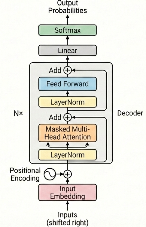
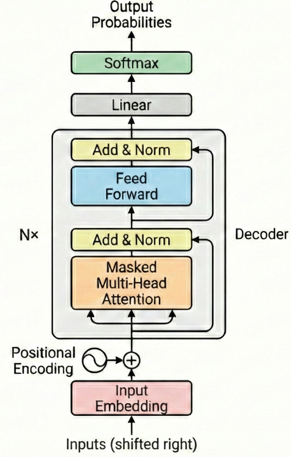
The Transformer architecture

Key components from last time:

• Self-attention with Q, K, V projections
• Multi-head attention for diverse relationships
• Causal masking for autoregressive generation
• Residual connections and layer normalization

• Quick review before we dive into implementation
• We covered the math; now we translate it to code
• Understanding tensor shapes is critical for Assignment 3

Recall: Scaled dot-product attention

\[ \text{Attention}(Q, K, V) = \text{softmax}\left(\frac{QK^\top}{\sqrt{d_k}}\right)V \]

Q

[n × d_k]

×

K^T

[d_k × n]

=

Scores

[n × n]

→

softmax

[n × n]

×

V

[n × d_v]

=

Output

[n × d_v]

• Q, K, V are linear projections of the input: \(Q = XW^Q\), \(K = XW^K\), \(V = XW^V\)
• Scaling by \(\sqrt{d_k}\) prevents softmax saturation
• Output for each position = weighted sum of all value vectors

• This is the formula you’ll implement step-by-step in Assignment 3
• Each step maps to one function in the notebook

Recall: Why scale by \(\sqrt{d_k}\)? Preventing softmax saturation

For random vectors \(\mathbf{q}, \mathbf{k} \in \mathbb{R}^{d_k}\) with entries ~ \(\mathcal{N}(0,1)\): \(\text{Var}(\mathbf{q} \cdot \mathbf{k}) = d_k\)

Without Scaling (d_k = 64)

Dot products have std dev ≈ 8

scores = [12, 8, 5, 1]

softmax ≈ [0.982, 0.018, 0.0, 0.0]

Near one-hot → vanishing gradients for non-max tokens

With Scaling: scores / √64 = scores / 8

Dot products rescaled to std dev ≈ 1

scaled = [1.5, 1.0, 0.625, 0.125]

softmax ≈ [0.439, 0.267, 0.183, 0.111]

Smooth distribution → healthy gradients for all tokens

• Without scaling, dot products grow proportionally to d_k
• Large dot products push softmax into saturation (near one-hot)
• Saturated softmax → near-zero gradients for non-max positions
• Dividing by √d_k restores unit variance, keeping softmax in a healthy operating range

Why \(\sqrt{d_k}\)? The variance argument

Assume \(q_i, k_i \sim \text{i.i.d.}\) with mean 0, variance 1. The dot product is:

\[ q \cdot k = \sum_{i=1}^{d_k} q_i \, k_i \]

Each term \(q_i k_i\) has: \(\;\mathbb{E}[q_i k_i] = 0\), \(\;\text{Var}(q_i k_i) = 1\)

By independence, the variance of the sum is:

\[ \text{Var}(q \cdot k) = \sum_{i=1}^{d_k} \text{Var}(q_i k_i) = d_k \]

So dot products grow as \(O(d_k)\). Dividing by \(\sqrt{d_k}\) restores unit variance:

\[ \text{Var}\!\left(\frac{q \cdot k}{\sqrt{d_k}}\right) = \frac{d_k}{d_k} = 1 \]

• Without scaling, larger d_k → larger dot products → softmax saturation → vanishing gradients
• It’s essentially the same problem as sigmoid saturation in old deep networks that motivated the switch to ReLU — just showing up in a different place in the architecture. The dk dk​​ scaling is the Transformer’s equivalent of careful initialization or batch norm for preventing activation saturation.

Recall: Multi-head attention and causal masking

Multi-head: Run \(h\) parallel attention operations with \(d_k = d_{model}/h\)

\[ \text{MultiHead}(Q, K, V) = \text{Concat}(\text{head}_1, \ldots, \text{head}_h)W^O \]

Causal masking: Prevent attending to future tokens

\[ \text{Attention}(Q, K, V) = \text{softmax}\left(\frac{QK^\top + M}{\sqrt{d_k}}\right)V \]

\[ \text{where } M_{ij} = \begin{cases} 0 & j \leq i \\ -\infty & j > i \end{cases} \]

Multi-head

Each head learns different relationships

Causal mask

Lower-triangular: token i sees only ≤ i

Transformer block

Attn + FFN + residuals + LayerNorm

• These three ideas combine into the full transformer block
• Now let’s see how to implement all of this in PyTorch

The decoder-only transformer block

Pre-Norm

Post-Norm

• The same block is stacked N times (e.g., N=12 in GPT-2, N=32 in LLaMA-7B)
• Modern LLMs use only this decoder stack — no separate encoder
• This is the decoder-only architecture used by GPT, LLaMA, Claude
• Each block: masked self-attention → add & norm → FFN → add & norm
• Residual connections (orange) bypass each sub-layer, enabling gradient flow
• The causal mask inside attention prevents looking at future tokens
• The LM head at top maps final hidden states to vocabulary probabilities

The Pre-Norm Decoder-only Transformer

• Show residuals and layer norms in more detail
• Post-Norm: output = LayerNorm(x + Sublayer(x))
• Pre-Norm: output = x + Sublayer(LayerNorm(x))

Part 1: Implementing Self-Attention

Tensor dimensions throughout attention

Input: \(X \in \mathbb{R}^{B \times n \times d_{model}}\)

Step	Operation	Shape
Input	X	(B, n_tok, d_model)
Project Q	Q = X @ W_Q	(B, n_tok, d_model)
Attention scores	A = Q @ K.T	(B, n_tok, n_tok)
Scale + Softmax	A = softmax(A / √d)	(B, n_tok, n_tok)
Output	O = A @ V	(B, n_tok, d_model)

• B = batch size, n_tok = sequence length, d_model = embedding dimension
• The attention matrix is n_tok × n_tok—this is where O(n²) comes from

• B is the batch dimension—we process multiple sequences in parallel
• The n × n attention matrix stores all pairwise attention weights
• Understanding these shapes is essential for implementing attention

Attenion as a block diagram

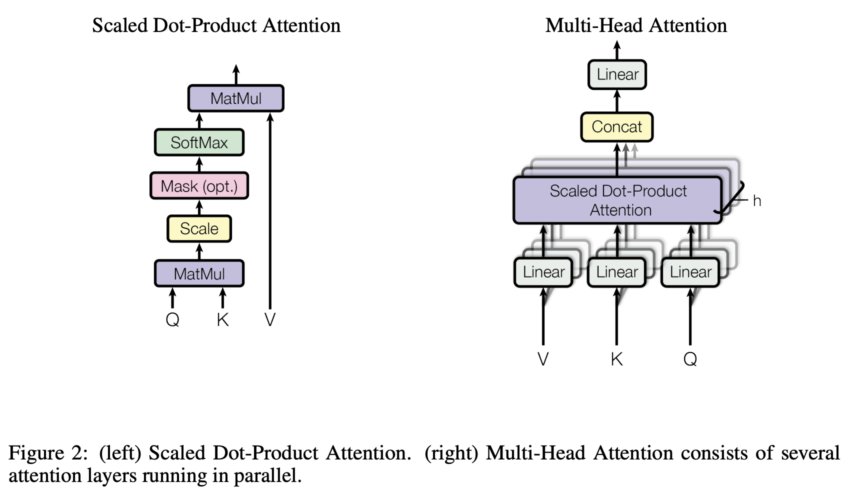
Multi-head attention — why split heads?

Problem: Single attention head has limited expressiveness

Solution: Run h parallel attention operations with smaller dimensions

Single Head

d_model = 512
1 attention operation

→

8 Heads

d_head = 512/8 = 64
8 parallel attention ops

• Same total parameters: one 512-dim head ≈ eight 64-dim heads
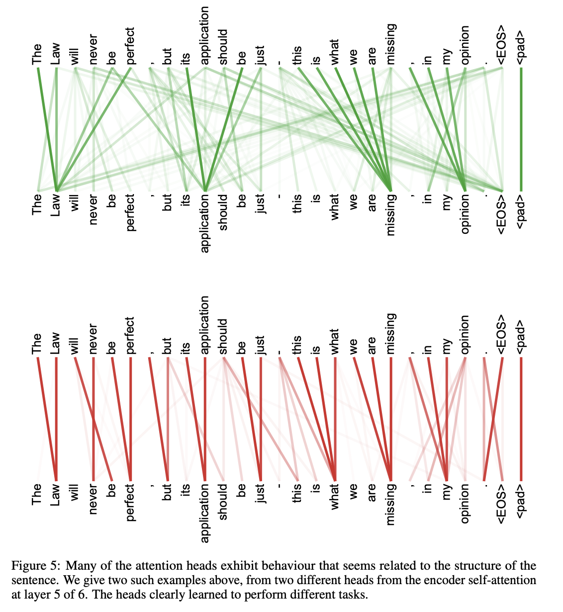
• Each head can learn different relationship types

• Multi-head attention doesn’t add parameters—it restructures them
• The key insight: d_model = n_heads × d_head
• Each head operates independently, then results are concatenated

Part 2: What Makes a Language Model “Large”

A language model predicts probability distributions over tokens

Core function:

\[ P(x_t \mid x_1, \ldots, x_{t-1}; \theta) \]

The cat sat on the

→

Transformer
(θ = parameters)

→

P(next token)

mat: 0.15
floor: 0.12
rug: 0.08
...

The model maps context → probability distribution over vocabulary

• This is the same objective as n-gram models, but with neural parameterization
• The transformer architecture computes this probability efficiently
• All the complexity serves this simple goal

“Large” refers to both parameters and training data

Model	Parameters	Training Tokens	Year
GPT-2	1.5B	40B	2019
GPT-3	175B	300B	2020
LLaMA-2	70B	2T	2023
GPT-4	~1.8T*	~13T*	2023

*Estimated, not officially disclosed

Scale has grown ~1000× in 4 years

• The trend has been dramatic increases in both dimensions
• Chinchilla (2022) showed data scaling was underemphasized
• Modern models use trillions of tokens

The three-stage training pipeline

1

Pretraining

Next-token prediction on massive corpora

Trillions of tokens
Weeks of compute

→

2

Instruction Tuning

Supervised fine-tuning on instruction-response pairs

Thousands of examples
Hours of compute

→

3

RLHF

Reinforcement learning from human feedback

Preference data
Days of compute

• Each stage serves a different purpose
• Pretraining: acquire knowledge and capabilities
• Instruction tuning: learn to follow instructions
• RLHF: align with human preferences for helpfulness and safety

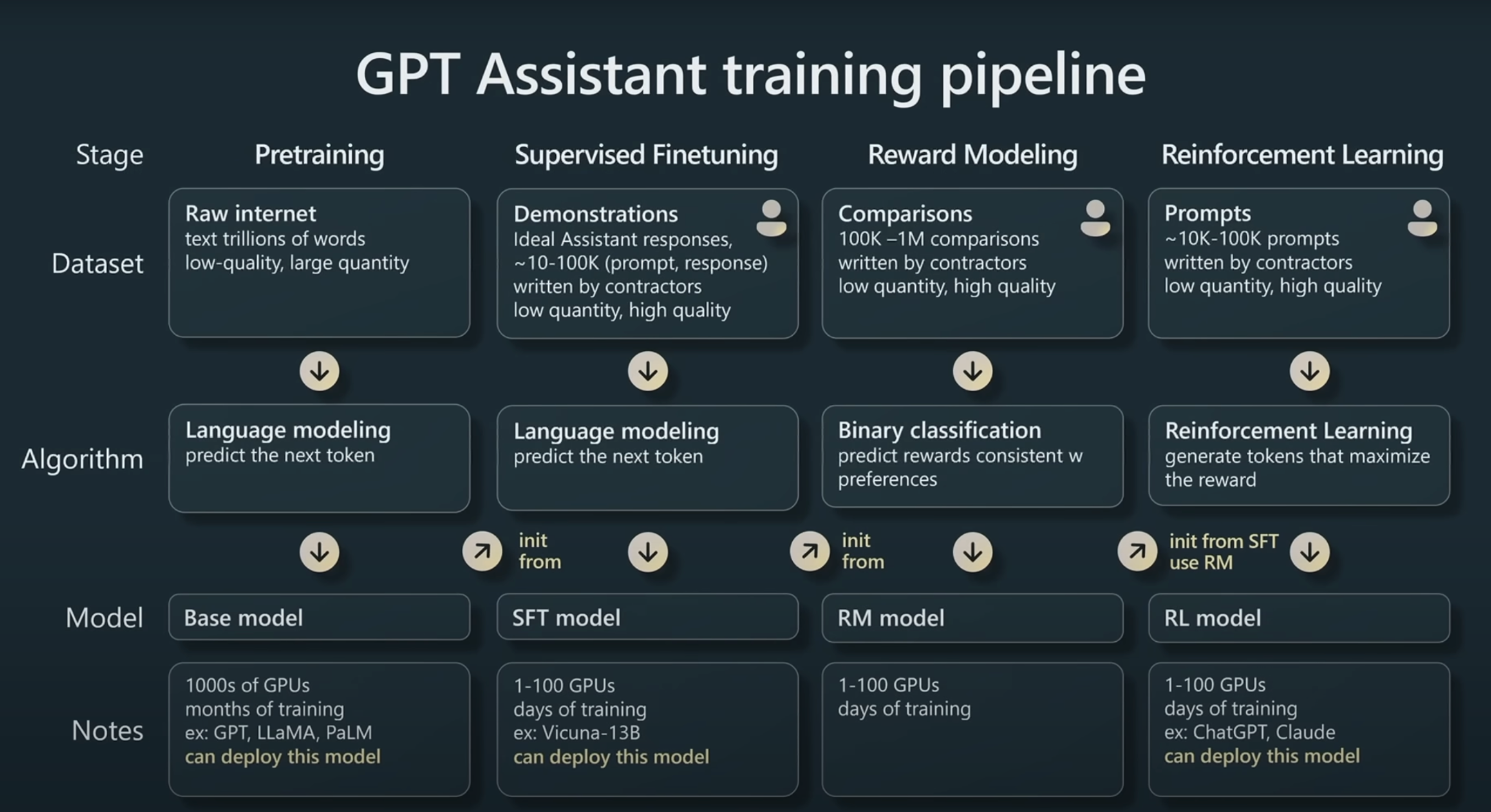
Slide from Andrej Karpathy: State of GPT

Part 3: Pretraining at Scale

The pretraining objective: predict the next token

Causal Language Modeling (CLM) loss:

\[ \mathcal{L}(\theta) = -\sum_{t=1}^{T} \log P_\theta(x_t \mid x_1, \ldots, x_{t-1}) \]

Training Example: "The quick brown fox jumps"

Context	Target	Loss contribution
<bos>	The	−log P(The | <bos>)
The	quick	−log P(quick | The)
The quick	brown	−log P(brown | The quick)
The quick brown	fox	−log P(fox | The quick brown)
The quick brown fox	jumps	−log P(jumps | ...)

• This is the same cross-entropy loss used throughout the course
• Each position provides a training signal
• The model learns to predict every word from its context

Self-supervision: the data labels itself

Traditional Supervised Learning

Image → Human labels "cat"

Requires expensive manual annotation

Self-Supervised (LLMs)

"The cat" → Next word is "sat"

Labels come from the text itself—free and unlimited

Key insight: The structure of language provides free supervision at massive scale

• This is why LLMs can train on trillions of tokens
• No human annotation needed for pretraining
• The same text provides |tokens| training examples

Next-token prediction implicitly learns many skills

To predict the next token well, the model must learn:

Grammar & Syntax

"She runs" not "She run"

World Knowledge

"Paris is the capital of France"

Reasoning Patterns

"If A then B. A is true. Therefore B"

Style & Tone

Formal vs. casual, technical vs. simple

The simple objective captures complex structure

• This is the “unreasonable effectiveness” of language modeling
• The model must understand the world to predict text about it
• Grammar, facts, reasoning—all emerge from the same objective

GPT-2 Paper

• This was not obvious at the time—many expected next-token prediction to be too simple
• GPT-2’s surprising capabilities sparked the current wave of research
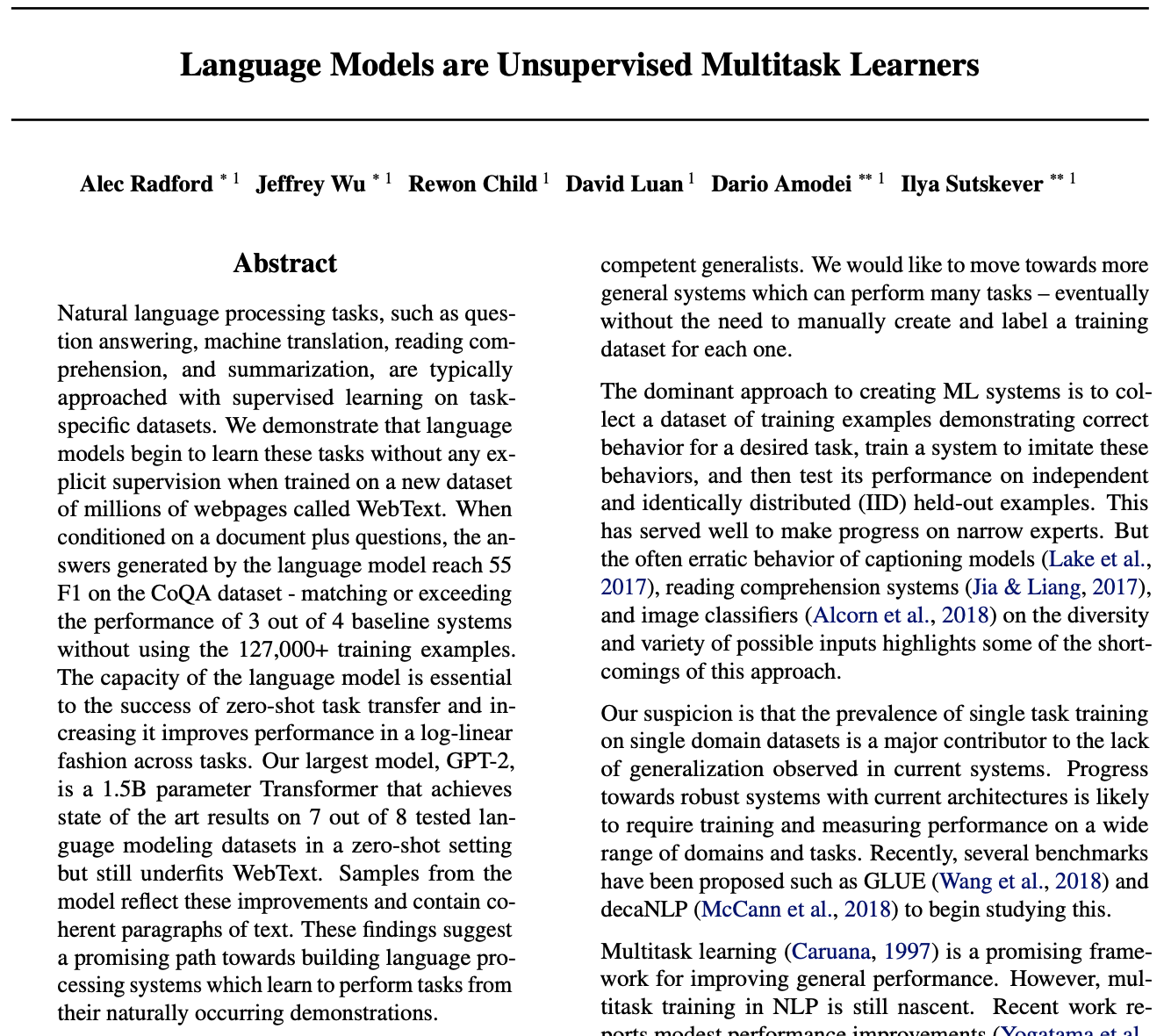
• The scaling laws we’ll discuss next were first observed in this paper

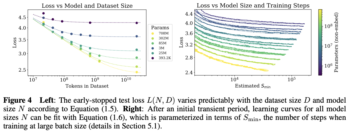
Scaling laws describe predictable improvement with resources

Empirical finding (Kaplan et al., 2020; Hoffmann et al., 2022):

\[ L(N, D) \approx \left(\frac{N_c}{N}\right)^{\alpha_N} + \left(\frac{D_c}{D}\right)^{\alpha_D} + L_\infty \]

N = Parameters

More parameters → lower loss

D = Data (tokens)

More data → lower loss

C = Compute

More FLOPs → lower loss

Loss decreases as a power law in each resource

• Constants: From the Kaplan et al. paper, the fitted values were approximately:

Nc​≈8.8 E 13 Dc​≈5.4 E 13 αN​≈0.076 αD​≈0.095

• The loss function L(N,D)L(N, D) L(N,D) has three terms:

(Nc​/N)αN​: Loss contribution from limited parameters. As N grows, this term shrinks — bigger models do better. NcN_c Nc​ and αN_N αN​ are empirically fitted constants.

(Dc​/D)αD​: Loss contribution from limited data. As D (tokens) grows, this term shrinks.

L∞​: The irreducible loss — the theoretical floor you’d hit with infinite parameters and infinite data. This represents inherent noise/entropy in language itself. You can never get loss below this.

The key insight is that both terms follow power laws — straight lines on a log-log plot. Performance doesn’t improve linearly with resources; you get diminishing returns, but the returns are predictable. - This is why “just scale it up” has been so effective - The relationships are smooth and predictable - Enables planning large training runs before starting

Scaling law curves (Kaplan et al., 2020)

Chinchilla scaling: balance parameters and data

Key insight (Hoffmann et al., 2022):

For a fixed compute budget, there’s an optimal ratio:

\[ N_{\text{opt}} \propto C^{0.5}, \quad D_{\text{opt}} \propto C^{0.5} \]

Rule of thumb: Train on ~20 tokens per parameter

Undertrained

70B params, 300B tokens

GPT-3 (4 tokens/param)

Compute-Optimal

70B params, 1.4T tokens

Chinchilla (20 tokens/param)

Inference-Optimal

7B params, 2T tokens

LLaMA (285 tokens/param)

• GPT-3 was likely undertrained by this analysis
• Chinchilla matched GPT-3 with 4× fewer parameters
• For deployment, smaller models with more training may be preferred
• That compute could have been used to train a larger model to lower loss.
• But LLaMA’s logic is: training happens once, inference happens millions of times. A 7B model that’s 95% as good as a 70B model but 10x cheaper to serve is a better business decision. You “waste” some training compute to get a smaller, cheaper model that’s still very good.