Interpretability: From Mechanistic Foundations to Practice

Robert Minneker

2026-02-26

Sources & Objectives

Key References: Elhage et al. (2021) — Transformer Circuits; Olsson et al. (2022) — Induction Heads; Bricken et al. (2023) — Monosemanticity; Templeton et al. (2024) — Scaling Monosemanticity; nostalgebraist (2020) — Logit Lens

By the end of this lecture, you will be able to:

1. Trace a computation through zero-, one-, and two-layer transformer circuits
2. Apply the logit lens and sparse autoencoders to inspect model internals at scale
3. Distinguish representational evidence (probes) from causal evidence (patching)
4. Evaluate when mechanistic understanding is necessary vs. when behavioral testing suffices
5. Honestly assess what interpretability can and cannot deliver today

• This companion lecture takes a bottom-up approach: start from the smallest circuits and build toward practice
• Contrast with the audit/triage framing of the previous lecture — here we build from mechanisms up
• Key thread: circuits are the atoms; scaling requires new tools; practice demands honest limits

This course builds an LLM engineering toolkit across six dimensions

Building

✓

Inference-Time Control

Prompting, decoding, self-consistency

✓

Training-Time Control

SFT/PEFT, continued pretraining, pref. tuning

✓

System-Time Augmentation

RAG, tools, agents

Understanding & Governing

TODAY

Understanding

Interpretability, causal methods

Measuring

Evaluation, contamination, protocols

Governing & Shipping

Safety engineering, deployment constraints

• Today we continue the Understanding dimension, now building from mechanistic foundations upward
• Previous lecture: top-down audit framing. This lecture: bottom-up circuit theory to practice

What question are you actually asking?

Three levels of interpretability questions, from surface to mechanism:

1. Behavioral

"What does the model do?" — Input-output testing, benchmarks, red teaming

2. Representational

"What does the model know?" — Probes, logit lens, feature visualization

3. Mechanistic

"How does the model compute?" — Circuits, activation patching, path tracing

This lecture builds bottom-up: start from mechanisms (circuits), develop scaling tools (probes, SAEs), then ask what practice demands.

Running themes:  1. Circuits are the atoms of understanding  2. Scaling requires new tools, not just more patience  3. Practice demands honest limits

• These three levels correspond roughly to Marr’s computational/algorithmic/implementation levels
• Most deployed interpretability today is behavioral. Mechanistic is the frontier.
• The bottom-up approach lets us see what the theory actually delivers before making practical claims

Part 1: Mechanistic Foundations

From tokens to circuits

We start at the simplest possible transformer computation — no attention, no MLPs — and build toward multi-layer circuits. Each step adds exactly one new mechanism.

• Part 1 covers the core circuit theory from Elhage et al. (2021) “A Mathematical Framework for Transformer Circuits”
• We build from zero layers to two layers, showing how complexity compounds

Zero-layer circuits: What does a transformer predict with no computation?

The simplest “circuit” — skip all attention heads and MLPs, go directly from input to output:

The zero-layer path

\[\text{logits} = W_U^T \cdot W_E \cdot x\]

\(W_E\): token embedding matrix
\(W_U\): unembedding matrix
\(x\): one-hot input token

What this captures

The product \(W_U^T W_E\) is a token-to-token matrix: row \(i\), column \(j\) gives the direct contribution of input token \(j\) to predicting output token \(i\).

This encodes bigram statistics — the model's baseline expectation of what follows what.

Input →	the	cat	sat	on
Top prediction	cat	is	on	the

• Elhage et al. (2021) call this the “direct path” through the residual stream
• The zero-layer model is essentially a bigram model learned from the training distribution
• Surprisingly informative baseline: you can read off what the model “expects” before any computation
• Key insight: every layer’s contribution is added to this baseline via the residual stream

Single-layer circuits: How does one attention head transform the zero-layer predictions?

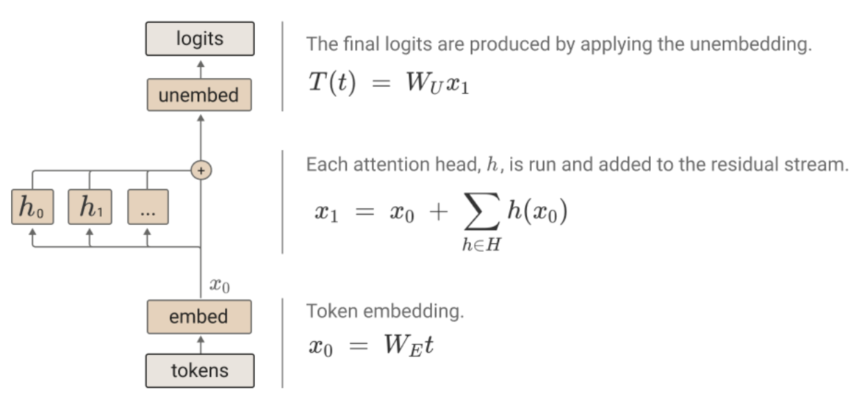
Source: Elhage et al., “A Mathematical Framework for Transformer Circuits” (2021)

• This figure from Elhage et al. (2021) shows the one-layer attention-only transformer
• Key equation: \(x_1 = x_0 + \sum_{h \in H} h(x_0)\) — each head’s output is added to the residual stream
• The token embedding gives \(x_0 = W_E t\), and the final logits are \(T(t) = W_U x_1\)
• Note the additive structure: the model’s output is the zero-layer baseline plus the sum of all head contributions

Single-layer circuits: Mathematical reformulation

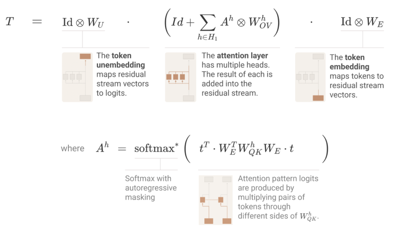
Source: Elhage et al., “A Mathematical Framework for Transformer Circuits” (2021)

• This reformulation expresses the entire single-layer transformer as a product of three terms
• Right term (token embedding): maps tokens to residual stream vectors
• Middle term (attention layer): identity plus the sum of all head contributions — each head applies an attention pattern \(A^h\) and a value transformation \(W_{OV}^h\)
• Left term (token unembedding): maps residual stream vectors back to logits
• The attention pattern logits are produced by multiplying pairs of tokens through different sides of \(W_{QK}^h\)

Single-layer circuits: Mathematical reformulation (cont.)

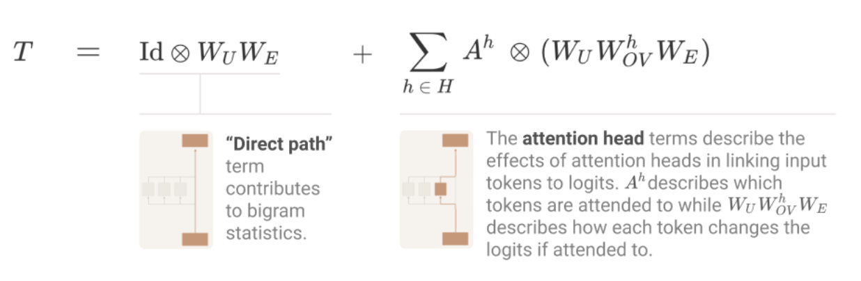
Source: Elhage et al., “A Mathematical Framework for Transformer Circuits” (2021)

• Multiplying out the previous expression gives two terms
• The “direct path” term \(\text{Id} \otimes W_U W_E\) is exactly the zero-layer circuit we saw earlier — bigram statistics
• Each attention head term \(A^h \otimes (W_U W_{OV}^h W_E)\) has two independent parts: where to attend (\(A^h\)) and what effect attending has (\(W_U W_{OV}^h W_E\))
• This separation is what motivates the QK/OV decomposition on the next slide

Splitting attention head terms into QK and OV circuits

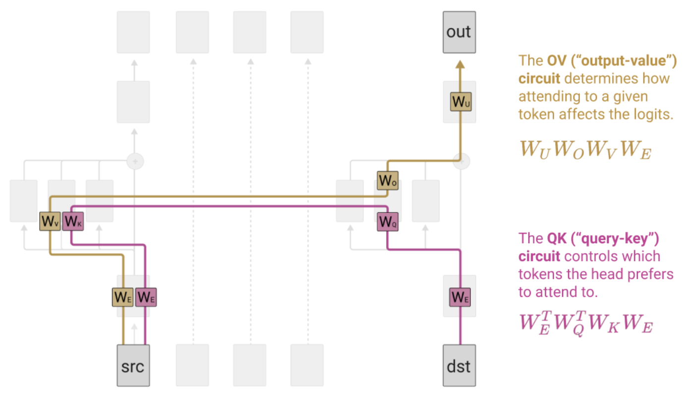
Source: Elhage et al., “A Mathematical Framework for Transformer Circuits” (2021)

• This diagram traces the full information flow through a single attention head
• The OV circuit (gold path): src token → \(W_E\) → \(W_V\) → \(W_O\) → \(W_U\) → output logits — this is “what happens when you attend to a token”
• The QK circuit (pink path): dst token → \(W_E\) → \(W_Q\) and src token → \(W_E\) → \(W_K\) — this is “which tokens attend to which”
• These two circuits are mathematically independent: you can analyze them separately
• This is the key insight that makes single-head interpretability tractable

QK and OV circuits: The atomic units of attention heads

Each attention head decomposes into two independent circuits:

QK Circuit — "Where to look"

\[A = \text{softmax}\!\left(\frac{x^T W_Q^T W_K x}{\sqrt{d_k}}\right)\]

Determines attention pattern: which source positions does each destination attend to?

OV Circuit — "What to move"

\[\text{output} = A \cdot x \cdot W_V W_O\]

Determines what information gets read from the attended position and how it's written to the residual stream.

Key insight (Elhage et al., 2021): A single attention head is the atomic unit of transformer computation. The QK and OV circuits can be analyzed independently — this is what makes mechanistic interpretability tractable at the single-head level.

• The QK circuit is a bilinear form — it computes compatibility between positions
• The OV circuit is a linear map — it reads from attended positions and writes to residual stream
• This decomposition is exact, not an approximation — it follows directly from the math of attention
• The full matrix \(W_Q^T W_K\) can be eigendecomposed to understand what token features determine attention

Induction heads and name movers: One-layer circuit motifs

The induction head circuit — the mechanistic basis of in-context learning:

Name Mover Heads (Wang et al., 2022)

In the IOI circuit ("When Mary and John went to the store, John gave a drink to ___"): name mover heads attend to "Mary" and copy it to the final position. This is a three-layer circuit with ~26 heads playing distinct roles.

• Induction heads: Olsson et al. (2022) showed these emerge abruptly during training in some settings
• Ablating induction heads substantially reduces in-context pattern-copying (strongest evidence in smaller models)
• Name movers: Wang et al. (2022) “Interpretability in the Wild” — the IOI circuit is the most complete circuit reverse-engineering to date
• IOI = Indirect Object Identification task

Activity: Compute a zero-layer prediction

Pair Activity (2 min)

Given this (simplified) bigram table from \(W_U^T W_E\):

Input ↓ / Output →	the	cat	sat	on
the	0.1	2.4	0.8	0.3
cat	1.1	0.2	2.7	0.6
sat	0.5	0.3	0.1	3.1
on	2.9	0.7	0.4	0.2

1. What does the zero-layer model predict after “the”? After “sat”?
2. Why is this a useful baseline for understanding what attention heads add?

• Answer: “the” → “cat” (logit 2.4), “sat” → “on” (logit 3.1)
• These are bigram predictions — no context, just token-to-token associations
• Everything attention heads and MLPs contribute is added to these baseline logits via the residual stream
• This is why the zero-layer model matters: it defines what the model predicts “for free”

Two-layer composition: How circuits chain together

When one head’s output becomes another head’s input, three types of composition arise:

Q-Composition

Head A's output is read by Head B's query — changes where Head B attends based on what Head A found.

K-Composition

Head A's output is read by Head B's key — changes what positions become attended based on Head A's computation.

V-Composition

Head A's output is read by Head B's value — changes what information gets moved at positions Head B already attends to.

Example: The induction circuit is K-composition — the previous-token head writes to the residual stream, and the induction head reads it via its key, changing which positions match the current query.

• These three composition types are exhaustive: any interaction between two heads must go through Q, K, or V
• Elhage et al. (2021) showed how to compute the effective circuit by multiplying the relevant weight matrices
• The induction head is a concrete example: Head 1 writes “what came before A” into the residual stream; Head 2’s keys now match positions that follow A
• This is where interpretability gets hard: two heads compose simply, but three or more layers create exponentially many paths

The residual stream: A shared communication bus

• The residual stream is a high-dimensional shared workspace — every layer reads from it and writes back to it
• Each layer’s contribution is additive: \(x_{out} = x_{in} + \text{Attn}(x) + \text{MLP}(x)\)
• This additive structure is why we can decompose the model into circuits at all

Theme 1: Circuits are the atoms of understanding — the residual stream is what makes them composable.

• The residual stream is the key architectural feature that makes transformer circuits analyzable
• nostalgebraist (2020) was one of the first to exploit this: project the residual stream at any layer into vocabulary space
• Without residual connections, the model would be a deep nonlinear pipeline with no natural decomposition
• The additive structure means we can attribute the final output to specific layers, heads, and even individual terms

The combinatorial wall: Why circuit analysis doesn’t simply scale

As models grow, the number of possible interaction paths explodes:

Model	Layers	Heads/Layer	Total Heads	2-Head Paths	All Paths
GPT-2 Small	12	12	144	~10K	~106
GPT-2 XL	48	25	1,200	~700K	~1026
Llama 70B	80	64	5,120	~13M	~10100+

• You cannot enumerate all circuits in a frontier model — the combinatorics are astronomical
• This motivates every tool in Part 2: we need methods that bypass exhaustive circuit search

Theme 2: Scaling requires new tools, not just more patience.

• The “all paths” count includes paths of all lengths through all possible subsets of heads
• Even 2-head paths (the simplest multi-head interaction) number in the millions for large models
• This is why the field shifted from hand-tracing circuits to automated methods (SAEs, activation patching)
• The honest takeaway: full mechanistic understanding of frontier models is currently out of reach

Part 2: Scaling Tools

From circuits to scalable methods

Since we can’t trace every circuit by hand, we need tools that summarize internal computation. Each tool trades off fidelity for scalability.

• Part 2 covers the practical toolkit: logit lens, probes, SAEs, patching
• Each tool is positioned on the continuum from “cheap but shallow” to “expensive but causal”

The logit lens: Reading the residual stream as vocabulary predictions

Idea (nostalgebraist, 2020): At every layer, project the residual stream through the unembedding matrix to see what the model would predict if it stopped here.

• nostalgebraist (2020) introduced this technique in the blog post “interpreting GPT: the logit lens”
• The key insight: because the residual stream is additive, you can meaningfully project intermediate states into vocabulary space
• Observation: early layers often predict syntactically plausible tokens; later layers refine to semantically correct ones
• Limitation: the unembedding matrix was trained for final-layer representations, not intermediate ones

Tuned lens: Fixing the logit lens’s calibration problem

Logit Lens Limitation

The unembedding matrix \(W_U\) was trained for final-layer representations. Early-layer projections are miscalibrated — they overestimate certainty on wrong tokens.

Early-layer residual stream representations live in a different subspace than the final layer expects.

Tuned Lens Fix (Belrose et al., 2023)

Train a learned affine probe per layer:

\[\hat{p}_l = \text{softmax}(W_U \cdot (A_l h_l + b_l))\]

Each \(A_l, b_l\) is trained to align layer \(l\)'s representation space with the final unembedding. Only the affine parameters are learned; the model is frozen.

• Tuned lens gives better-calibrated predictions at every layer, especially in early/middle layers
• Reveals a cleaner picture of when the model forms its predictions

• Belrose et al. (2023) “Eliciting Latent Predictions from Transformers with the Tuned Lens”
• The affine transformation is small (only d_model + 1 parameters per layer) — it corrects the representation basis, not learning new features
• In practice, tuned lens predictions converge to the final answer earlier than logit lens predictions
• This matters for understanding where in the network specific knowledge is stored/computed

Probing classifiers: What is linearly decodable from representations?

Setup: Train a linear classifier on frozen embeddings: \(y_i = \text{softmax}(Wh_i + b)\)

Frozen Model

BERT, GPT, etc.

→

Embedding h_i

Per token

→

Linear Probe

Predicts label y_i

Decodability

Information is linearly extractable from the representation. Cheap, scalable. BERT middle layers encode syntax best; upper layers encode semantics (Tenney et al., 2019).

≠ Causal Use

High probe accuracy does not mean the model uses that information. Hewitt & Liang (2019): use control tasks + selectivity. Amnesic probing (Elazar et al., 2021) removes information to test causal role.

• Probes are the workhorse of representational analysis — fast to train, applicable at scale
• The decodability vs. causal use distinction is critical: just because you can read POS tags from layer 6 doesn’t mean the model computes POS tags
• Control tasks (probing random labels) help calibrate whether probe accuracy is meaningful
• Amnesic probing: project out the probe’s direction and see if downstream performance drops — bridges representational and causal evidence

Activity: Sketch a logit lens for “The Eiffel Tower is in”

Individual + Compare (3 min)

For the input “The Eiffel Tower is in”, sketch what you think the logit lens top-1 prediction would be at each layer:

Layer	Embedding	Layer 2	Layer 6	Layer 10	Layer 12	Final
Top-1	?	?	?	?	?	?
Confidence	low	?	?	?	?	high

1. Fill in your guesses, then compare with a neighbor
2. At what layer do you think “Paris” first appears as the top prediction?

• Typical pattern: embedding layer predicts something generic (“the”, “a”); middle layers start to form “France” or “Paris”; final layers lock onto “Paris”
• Students often expect “Paris” to appear immediately — the gradual convergence is the key insight
• In practice on GPT-2, factual knowledge tends to crystallize in middle-to-late layers
• This exercise builds intuition for the tuned lens slide that follows

Sparse autoencoders decompose superposed features into interpretable units

Superposition problem: Models encode more features than they have dimensions, causing features to overlap.

Without Disentangling

Neuron 42 fires for "France," "cheese," and "revolution" — polysemantic

With Sparse Autoencoder

Feature 107 = "France (country)", Feature 238 = "dairy products" — monosemantic

SAE objective — reconstruct activations with sparse features:

\[\mathcal{L} = \| h - \hat{h} \|_2^2 + \lambda \| z \|_1\]

where \(\hat{h} = W_{dec} \cdot \text{ReLU}(W_{enc} \cdot h + b_{enc}) + b_{dec}\) and \(z\) are the encoder activations.

• Reconstruction term (\(L_2\)): features should faithfully reconstruct the original activation
• Sparsity penalty (\(L_1\)): only a few features should be active for any given input
• Bricken et al. (2023): thousands of interpretable features from Claude’s MLP layers
• Templeton et al. (2024): scaled to Claude 3 Sonnet — millions of interpretable features

• The L1 penalty is the key: it forces the autoencoder to find a sparse basis, breaking superposition
• The decoder columns become the “feature directions” in activation space
• Bricken et al. found features for specific concepts: Golden Gate Bridge, code bugs, legal language
• Templeton et al. showed this scales: more features = more fine-grained concepts, following scaling laws
• Limitation: some residual polysemanticity remains; automated labeling introduces its own errors

Activation patching and path patching: Causal tools for circuit discovery

Activation patching: Replace one activation with a value from a different context; measure the output change.

Clean Run

Normal activations

→

Patch a_l,i

From corrupted run

→

Measure Δy

Large Δy = causal

Path patching extends this to trace specific information routes:

Activation Patching

Patch all outputs of a component (head, layer, MLP). Tells you what matters.

Path Patching

Patch the output of component A only as read by component B. Tells you how information flows between specific components.

• Path patching was critical for the IOI circuit discovery (Wang et al., 2022) — identified which heads read from which other heads

• Activation patching is an intervention (Pearl’s do-calculus): do(a_l = a_l_corrupt) and measure the effect
• This is the closest analog to controlled experiments we have for neural networks
• Path patching adds specificity: instead of “head 9.1 matters,” you learn “head 9.1 reads from head 7.3 via V-composition”
• The IOI circuit paper used path patching to map the full 26-head circuit for indirect object identification
• Cost: each patch requires a forward pass — O(components × paths) for full path patching

The evidence hierarchy: Not all interpretability evidence is equal

5. Path Patching

Traces causal flow between specific components

STRONGEST

4. Activation Patching

Causal effect of a component on output

CAUSAL

3. Probing + Control Tasks

Decodability with selectivity baseline

CONTROLLED

2. Attention Visualization / Logit Lens

Descriptive, correlational, suggestive

DESCRIPTIVE

1. Behavioral Testing Only

Input-output, no internal access

WEAKEST

• This hierarchy is a simplification — each level has appropriate use cases
• Behavioral testing is often sufficient and most practical for deployed systems
• The key question is: what level of evidence does your application actually need?
• Safety-critical systems may need causal evidence; product monitoring may only need behavioral

Part 3: Bridging to Practice

From understanding to deployment

Mechanistic knowledge is only useful if it changes what you do. This section asks: when does circuit-level understanding actually help in practice?

• Part 3 transitions from research tools to deployment considerations
• The central tension: mechanistic interpretability is deep but expensive; behavioral testing is shallow but practical

Steering vectors: Editing model behavior via representations

Core idea: Find a direction in activation space that corresponds to a concept, then add or subtract it at inference time.

\[v_{\text{steer}} = \text{mean}(h_{+}) - \text{mean}(h_{-})\]

where \(h_+\) are activations from positive examples and \(h_-\) from negative examples.

Computing the Vector

1. Collect activations on "honest" prompts → \(h_+\)
2. Collect activations on "deceptive" prompts → \(h_-\)
3. Difference of means = steering direction

Applying the Vector

At layer \(l\): \(h_l' = h_l + \alpha \cdot v_{\text{steer}}\)
\(\alpha > 0\): amplify the concept
\(\alpha < 0\): suppress the concept
No retraining required — inference-time only

Examples from representation engineering (Zou et al., 2023):

• Honesty/deception, positive/negative sentiment, refusal/compliance
• Works across many prompts, not just the training examples

Caveat: Steering vectors are a blunt instrument. They affect all inputs, not just the targeted behavior. Side effects on unrelated capabilities are common and hard to predict.

• Li et al. (2023) “Inference-Time Intervention” and Zou et al. (2023) “Representation Engineering” are the key references
• The connection to mechanistic interp: steering vectors work because concepts are linearly represented (the linear representation hypothesis)
• This is a bridge from understanding to control — if you can find a direction, you can edit behavior
• Limitation: the mean-difference approach assumes the concept is linearly separable, which may not hold for complex behaviors

Mechanistic red teaming: Using circuits to find failure modes

	Traditional Red Teaming	Mechanistic Red Teaming
Approach	Craft adversarial inputs, observe outputs	Identify vulnerable circuits, predict failure modes
Evidence	Behavioral (found an exploit)	Mechanistic (understand why it fails)
Scalability	Scales with human effort / automation	Currently limited to smaller models / specific circuits
Fixes	Patch the input (filter, RLHF)	Patch the circuit (ablation, steering, editing)
Maturity	Production-ready	Research stage

• The promise: if you understand why a model fails, you can anticipate new failure modes, not just patch known ones
• The reality: mechanistic red teaming currently works best on targeted, well-defined behaviors (bias in specific circuits, knowledge errors in specific MLPs)

• Traditional red teaming is the current standard: hire humans or use automated tools to find failures
• Mechanistic red teaming would let you say “this circuit for gender-occupation associations could produce biased outputs on inputs X, Y, Z” before you test those inputs
• Current state: promising on small models (e.g., finding bias circuits in GPT-2), not yet practical at frontier scale
• Hybrid approach is most realistic: use mechanistic insights to guide where traditional red teaming focuses

Activity: When is mechanistic understanding necessary?

Pair Debate (3 min)

For each scenario, argue: is behavioral testing sufficient, or do you need mechanistic understanding?

A. Customer-service chatbot for an e-commerce site

B. Medical diagnosis assistant recommending treatments

C. Content moderation system for a social platform

D. Research tool: "Does GPT-4 have a model of other agents' beliefs (theory of mind)?"

For each: What could go wrong? What level of evidence (from the hierarchy) do you need?

• A: Behavioral likely sufficient — low stakes, can monitor and retrain
• B: Strong argument for mechanistic — need to know WHY a recommendation is made, regulatory requirements
• C: Middle ground — behavioral for deployment, mechanistic for auditing bias circuits
• D: Requires mechanistic — behavioral tests can’t distinguish “has ToM” from “learned ToM-like shortcuts”
• The key insight: required evidence level depends on stakes and the nature of the question

Behavioral vs. mechanistic evidence: What does deployment require?

Behavioral Evidence

Strengths: Scalable, fast, applicable to any model, maps directly to user experience

Weaknesses: Can miss systematic failures, doesn't explain causes, vulnerable to dataset artifacts

Best for: Deployment monitoring, A/B testing, regression checks

Mechanistic Evidence

Strengths: Explains causes, can predict novel failures, enables targeted fixes

Weaknesses: Expensive, limited to smaller models/specific tasks, may not generalize

Best for: Safety audits, debugging specific failures, scientific understanding

Regulatory note: The EU AI Act (2024) requires "sufficient transparency" for high-risk AI systems, but does not mandate mechanistic interpretability specifically. The NIST AI RMF similarly emphasizes risk-proportionate transparency. In practice, behavioral testing + documentation currently satisfies most compliance requirements.

• This is the pragmatic slide: most deployed systems use behavioral evidence, and that’s often appropriate
• Mechanistic evidence is most valuable when you need to answer “why” — for safety audits, scientific claims, or debugging specific failures
• The EU AI Act Article 13 requires transparency proportional to risk level — this currently means documentation, testing, and monitoring rather than circuit analysis
• The field needs better bridges: mechanistic findings should inform what behavioral tests to run

Production interpretability: What ships today vs. what’s still research

Ships Today PRODUCTION

Feature attribution (SHAP, integrated gradients) · Attention visualization · Token-level saliency maps · Confidence calibration · Behavioral test suites

Emerging / Limited Deployment PILOT

SAE-based feature dashboards · Steering vectors for behavior control · Probing-based runtime monitoring · Activation anomaly detection

Research Only LAB

Full circuit reverse-engineering · Automated circuit discovery · Model editing (ROME/MEMIT) at scale · Formal verification of neural networks

• This taxonomy is approximate and evolving — some “emerging” tools may be in production at specific companies
• The key message: there’s a large gap between what the research literature demonstrates and what’s deployable
• SHAP and attention visualization are well-established but provide limited mechanistic insight
• SAE dashboards (e.g., Anthropic’s feature visualization tools) are moving toward deployment but aren’t standard yet

The production interpretability stack

A realistic 4-step workflow for incorporating interpretability into a deployed LLM system:

1. Pre-Deploy Audit

Behavioral test suites + probing for known risks (bias, factuality, safety). Establish baselines. Identify critical failure modes with targeted red teaming.

2. Runtime Monitoring

Confidence calibration, output distribution tracking, activation anomaly detection (if feasible). Flag outputs that deviate from expected patterns.

3. Incident Investigation

When failures occur: feature attribution → probing → activation patching (if needed). Escalate from behavioral to mechanistic evidence as needed.

4. Continuous Improvement

Feed findings back: update test suites, adjust steering vectors, retrain probes, fine-tune on failure cases. Close the loop.

Theme 3: Practice demands honest limits — the stack escalates from cheap/shallow to expensive/deep only as needed.

• This mirrors standard software debugging: start with logs and metrics, escalate to profiling and tracing
• Most production issues can be resolved at steps 1-2 without mechanistic analysis
• Step 3 (mechanistic investigation) is reserved for failures that behavioral evidence can’t explain
• Step 4 is critical and often missing: interpretability findings need to feed back into the pipeline

Part 4: Honest Assessment

Where are we, really?

Interpretability has made remarkable progress. It also has fundamental unsolved problems. This section is about being honest about both.

• Part 4 gives the field its honest due — what’s real, what’s hype, and what’s genuinely unknown
• Students should leave with calibrated expectations, not either cynicism or overconfidence

What works today

Circuits on Small Models

Complete circuit analysis for specific tasks on GPT-2 scale models. Induction heads, IOI circuit, greater-than circuit. These are real, validated, causal findings.

Olsson et al. 2022, Wang et al. 2022, Hanna et al. 2023

SAEs at Scale

Millions of interpretable features extracted from Claude 3 Sonnet. Feature steering demonstrably changes behavior. A breakthrough in dealing with superposition.

Bricken et al. 2023, Templeton et al. 2024

Behavioral Probing

Probes reliably identify what information is encoded where. Combined with control tasks, this is a mature methodology. Practical for deployment monitoring.

Belinkov 2022, Hewitt & Liang 2019

• These three categories represent genuine, solid progress
• Circuits work: the IOI circuit has been independently replicated and extended
• SAEs work: the Golden Gate Claude demonstration was a compelling proof of concept
• Probes work: decades of work in NLP probing has produced a reliable methodology
• But “works” needs qualification: circuits work on small models; SAEs produce some residual polysemanticity; probes show decodability, not necessarily causal use

Activity: Works / Open / Wishful Thinking

Rapid Vote — Whole Class (2 min)

For each claim, vote: Works (solid evidence), Open (active research, unclear), or Wishful (no good evidence yet).

1. "We can identify the circuit for any specific behavior in GPT-2."

2. "SAE features correspond to human-interpretable concepts."

3. "Mechanistic interpretability can prevent deceptive alignment."

4. "Probing tells us what the model 'believes.'"

5. "We'll have full mechanistic understanding of frontier models within 5 years."

(Show of hands for each. Instructor reveals suggested answers after all votes.)

• Suggested answers: 1 = Open (works for some behaviors, not arbitrary ones); 2 = Works (with caveats about residual polysemanticity); 3 = Wishful (no demonstration yet); 4 = Open (decodability ≠ belief; causal probing is closer); 5 = Wishful (the combinatorial wall makes this unlikely with current methods)
• The goal is to calibrate expectations — students who’ve just learned these exciting tools may overestimate their current reach
• Encourage disagreement — reasonable people disagree on 1 and 4 especially

Open problems: What the field hasn’t solved

Scaling

Circuit analysis works on GPT-2 (117M params). Frontier models are 100-1000x larger. No one has reverse-engineered a complete circuit in a 70B+ model.

Superposition

SAEs help, but we don't know if they fully resolve superposition. Features may have complex, non-linear interactions that sparse decomposition misses.

Validation

How do you verify that a discovered "circuit" is the real mechanism, not an artifact of your analysis method? Ground truth is rarely available.

Closing the Loop

Interpretability findings rarely lead to concrete model improvements. The field needs better workflows from "we understand X" to "we fixed Y."

• Scaling: the combinatorial wall from Part 1. Automated methods help but haven’t overcome it for frontier models
• Superposition: Toy models (Elhage et al. 2022 “Toy Models of Superposition”) show it’s a real phenomenon, but solving it completely is an open problem
• Validation: Without ground truth, we rely on consistency checks — but consistency can be misleading
• Closing the loop: this is perhaps the most important practical challenge — interpretability needs to be actionable
• Neel Nanda’s “200 Concrete Open Problems in Mechanistic Interpretability” is a great resource for students interested in research

The path forward

Hybrid Approaches

Use mechanistic insights to guide behavioral testing:

• Circuit analysis identifies a bias mechanism → design targeted behavioral tests
• SAE features flag anomalous activations → trigger deeper investigation
• Probing reveals unexpected encoding → validate with causal intervention

The two levels of evidence are complementary, not competing.

Automated Interpretability

Use models to interpret models:

• LLMs label SAE features (Bills et al., 2023)
• Automated circuit discovery (Conmy et al., 2023 — ACDC)
• Scalable oversight: models audit each other's internals

Promise: overcomes the human bottleneck. Risk: introduces new failure modes (LLM labelers can hallucinate).

• The hybrid approach is the most realistic near-term path: mechanistic insights inform behavioral testing priorities
• Automated interpretability is exciting but creates a recursive trust problem: how do you verify the interpreter’s interpretation?
• ACDC (Automatic Circuit DisCovery) by Conmy et al. (2023) automates the patching process to find circuits
• Bills et al. (2023) “Language models can explain neurons in language models” — GPT-4 labels GPT-2 neurons
• The case for interpretability as infrastructure: building reusable tools that make interpretability cheaper over time

Summary: Key Takeaways

1. Circuits (zero/one/two-layer) provide the mathematical foundation — the residual stream’s additive structure makes decomposition possible
2. The combinatorial wall is real — scaling from GPT-2 to frontier models requires fundamentally new approaches
3. Scaling tools (logit lens, probes, SAEs, patching) trade fidelity for tractability — know where each sits on the evidence hierarchy
4. Causal evidence (patching) is stronger than representational evidence (probes) is stronger than behavioral evidence (testing) — but each has its place
5. Practice demands honesty — production systems mostly use behavioral methods; mechanistic analysis is reserved for when you need to know why
6. The path forward is hybrid: mechanistic insights guiding behavioral tests, with automation closing the scalability gap

• These six points map to the lecture’s three themes: circuits as atoms, scaling requires new tools, practice demands honest limits
• The most important meta-lesson: match your interpretability method to the question you’re actually asking

Further Reading

References & Resources

1. Elhage et al., “A Mathematical Framework for Transformer Circuits” (Anthropic, 2021) — The foundational paper on QK/OV circuits and composition
2. Olsson et al., “In-context Learning and Induction Heads” (Anthropic, 2022) — Mechanistic explanation of in-context learning
3. Bricken et al., “Towards Monosemanticity” (Anthropic, 2023) — Sparse autoencoders for feature extraction
4. Templeton et al., “Scaling Monosemanticity” (Anthropic, 2024) — SAEs at Claude 3 Sonnet scale
5. nostalgebraist, “interpreting GPT: the logit lens” (2020) — The original logit lens blog post
6. Wang et al., “Interpretability in the Wild: IOI” (2022) — Most complete circuit reverse-engineering to date
7. Belrose et al., “Eliciting Latent Predictions with the Tuned Lens” (2023) — Calibrated layer-wise predictions
8. Zou et al., “Representation Engineering” (2023) — Steering vectors and concept directions
9. Conmy et al., “Towards Automated Circuit Discovery” (2023) — ACDC for scalable circuit finding

• Elhage et al. (2021) is the essential starting point — it introduces the mathematical framework for everything else
• For students interested in research, Neel Nanda’s “200 Concrete Open Problems in Mechanistic Interpretability” provides many accessible starting points

Coming Up Next

March 3: Evaluation and Benchmarking

• How do we measure what models can and can’t do?
• Contamination, data leakage, and the benchmark treadmill
• Designing evaluations that actually inform deployment decisions

• Next lecture moves from Understanding to Measuring in our toolkit
• The interpretability → evaluation connection: you need to know what to test, and interpretability can inform that