Finetuning and Adaptation

Robert Minneker

2026-02-19

Roadmap for our Final Push

Building

✓

Inference-Time Control

Prompting, decoding, self-consistency

TODAY

Training-Time Control

SFT/PEFT, continued pretraining, pref. tuning

System-Time Augmentation

RAG, tools, agents

Understanding & Governing

Understanding

Interpretability, causal methods

Measuring

Evaluation, contamination, protocols

Governing & Shipping

Safety engineering, deployment constraints

• Course roadmap showing six complementary dimensions of LLM engineering
• Row 1 covers building: inference-time → training-time → system-time control
• Row 2 covers understanding & governance: interpretability → evaluation → safety/deployment
• Today we focus on training-time control — adapting model weights via finetuning, LoRA, and preference tuning

Running Example: Building a Customer Support Chatbot

Throughout this lecture, we’ll follow a concrete scenario: adapting an LLM to serve as a customer support chatbot for an e-commerce company.

Scenario:

Company: An online retailer with 10K support tickets/day
Goal: Automate responses for order status, returns, and product questions
Data: 50K historical ticket-response pairs + product catalog
Constraints: Must match brand voice, never hallucinate order details, handle escalation

• As we cover each adaptation method, we’ll ask: how would you apply this to our chatbot?

• This running example will be referenced throughout the lecture to ground abstract concepts
• Students should think about which adaptation method best fits this scenario

Part 1: From Pretrained to Task-Specific

State Change: Why Adapt?

Pretrained LLMs are powerful but general-purpose. We need principled methods to specialize them for downstream tasks.

Pretrained LLMs need adaptation: the finetuning objective

Pretraining objective:

\[ \mathcal{L}_{\text{pretrain}} = -\sum_{t=1}^T \log p_\theta(w_t \mid w_{<t}) \]

Finetuning objective on labeled data \((x_i, y_i)\):

\[ \mathcal{L}_{\text{finetune}} = -\sum_{i=1}^N \log p_{\theta'}(y_i \mid x_i) \]

Pretrained θ

General knowledge

→

Task Data

(x, y) pairs

→

Adapted θ'

Task specialist

• Pretraining gives broad knowledge; finetuning on labeled (x, y) pairs specializes it for downstream tasks.

• What Pretraining Gives: Broad linguistic knowledge, world facts, reasoning patterns
• What’s Missing: Task-specific formats, domain expertise, instruction following
• Transfer learning: leverage pretrained representations, adapt to new distribution
• The key question: how much of the model should we update?

Full finetuning updates all parameters but risks catastrophic forgetting

\[ \theta^* = \arg\min_\theta \mathcal{L}_{\text{task}}(f(x; \theta), y) \]

• All layers modified: embeddings, attention, FFN, output heads
• Risk: Catastrophic forgetting — prior pretraining knowledge lost

1. Learning rate scheduling

Controls how aggressively weights change per step (warmup + decay)

2. Parameter-efficient methods (LoRA)

Controls which weights are allowed to change at all (freeze base, train small adapters)

3. Short training

Controls how many steps you take — early stopping before old knowledge is overwritten

4. Replay / Data mixing

Controls what data distribution you optimize for — mix pretraining data with task data to preserve general knowledge

We often combine mitigations: These are complementary strategies — tuning the learning rate, which layers update, how long you train, and what data you train on.

• Full finetuning is appropriate when task distribution differs substantially from pretraining; leads to the motivation for parameter-efficient methods

Part 2: Parameter-Efficient Finetuning (PEFT)

State Change: Efficient Adaptation

Full finetuning is expensive and risky. PEFT methods update only a small fraction of parameters while achieving competitive performance.

LoRA freezes pretrained weights and adds low-rank update matrices

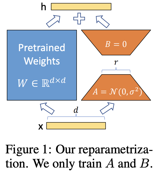
Key idea: Task-specific weight changes lie in a low-dimensional subspace.

\[ W = W_0 + \Delta W, \quad \Delta W \approx BA \]

Initialization: \(A\) is initialized with random Gaussian values; \(B\) is initialized to zero. This ensures \(\Delta W = BA = 0\) at the start of training, so the model begins from exactly the pretrained behavior.

• W₀ stays frozen — the original model is unchanged
• The low-rank hypothesis: most task-specific changes occupy a small subspace
• LoRA was proposed by Hu et al. (2021) and has become the dominant PEFT method
• The zero initialization of B is crucial: it means the adapted model starts identical to the pretrained model and gradually learns task-specific deviations
• The tall-thin B and short-wide A matrices have far fewer entries than the full d×d weight matrix
• At inference time, BA can be merged into W₀ with zero additional latency

LoRA achieves massive parameter savings with minimal performance loss

Method	Parameters per layer	Ratio
Full finetuning	16,777,216	100%
LoRA (r=8)	65,536	0.39%
LoRA (r=4)	32,768	0.20%

• Diminishing returns beyond moderate \(r\) (empirically \(r=4\) or \(r=8\) suffices)
• Many LoRA adapters can be swapped on a single base model for multi-task deployment
• Backpropagation is confined to small A and B matrices — much faster training

• The practical impact: hundreds of task-specific adapters on one pretrained LLM
• Common misconception: increasing r always improves performance — in practice it plateaus or even degrades

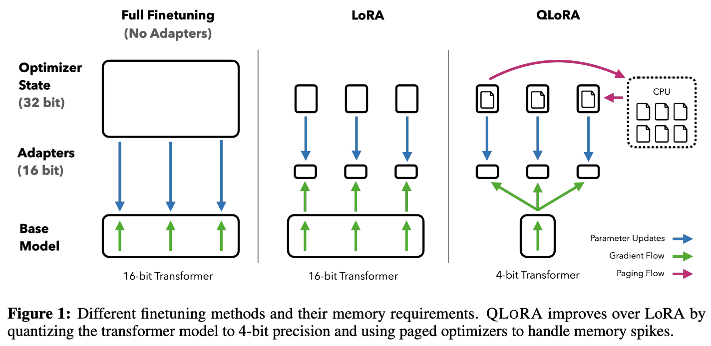
QLoRA: 4-bit quantization makes LoRA accessible on consumer hardware

QLoRA breakthrough: Dettmers et al. (2023) combined 4-bit quantization with LoRA, enabling finetuning of a 65B-parameter model on a single 48GB GPU — a task that previously required multiple high-end GPUs. This democratized access to large model finetuning.

• QLoRA stores the frozen base model in 4-bit precision while keeping LoRA adapters in full precision
• This 16x memory reduction makes it possible to finetune the largest open models on a single high-end GPU

QLoRA: 4-bit quantization makes LoRA accessible on consumer hardware

Worked Example: How much does LoRA actually save?

Setup: A transformer attention layer with \(d = 4096\), rank \(r = 8\)

\[\text{Full FT params per layer} = d^2 = 4096^2 = 16{,}777{,}216\] \[\text{LoRA params per layer} = 2 \times r \times d = 2 \times 8 \times 4096 = 65{,}536\] \[\text{Compression ratio} = \frac{65{,}536}{16{,}777{,}216} = 0.39\%\]

Note: Real transformer layers have rectangular weight matrices (e.g., MLP layers are \(d \times 4d\)). The \(d^2\) figure is illustrative for attention projections where \(d_{\text{model}} = d_{\text{head}} \times n_{\text{heads}}\).

For our chatbot:

A 7B-param model has ~32 attention layers × 4 weight matrices = 128 LoRA targets
Total LoRA params: 128 × 65,536 ≈ 8.4M trainable params (0.12% of 7B)
Training time: hours on a single GPU vs. days for full finetuning

• This calculation is a common interview question — students should be able to do it from memory
• The key insight: rank r=8 captures most task-specific variation; diminishing returns beyond r=16
• Recall the decision map — LoRA falls squarely in the “PEFT” quadrant: moderate domain shift, moderate data, limited compute

Why low-rank? The manifold hypothesis and intrinsic dimensionality

The manifold hypothesis: Natural data lies on low-dimensional manifolds embedded in high-dimensional space. By extension, the task-specific adjustments needed to adapt a pretrained model also occupy a low-dimensional subspace.

High-dimensional parameter space

A 7B model has billions of parameters, but task-specific changes don't need to move in all directions at once.

Low intrinsic dimensionality

Aghajanyan et al. (2021) showed the intrinsic dimensionality of finetuning is often just ~200–800, even for tasks with millions of parameters.

LoRA exploits this

By constraining ΔW = BA to rank r, LoRA is an inductive bias that says: "task adaptation lives in a small subspace." The data confirms this — r=8 suffices for most tasks.

• Larger pretrained models have lower intrinsic dimensionality for downstream tasks — the prior is stronger, so less adaptation is needed.

• Aghajanyan et al. (2021) “Intrinsic Dimensionality Explains the Effectiveness of Language Model Fine-Tuning” — the foundational paper connecting LoRA’s success to intrinsic dimensionality.
• This also explains why prompt tuning works at scale (Lester et al. 2021): at 10B+ params, the manifold of useful adaptations is so low-dimensional that even soft input tokens can navigate it.

PEFT Methods at a Glance

Method	Where it intervenes	Trainable params	Best for
LoRA	Weight matrices (Q, K, V, O, and commonly MLP layers)	0.1–1%	General default — most tasks
Adapters	Bottleneck layers in transformer blocks	1–5%	Multi-task deployment
Prefix Tuning	Learned K/V states prepended per layer	<0.1%	Generation tasks
Prompt Tuning	Soft tokens at input embeddings	<0.01%	Scales with model size (Lester et al. 2021: matches finetuning at 10B+ params)
QLoRA	4-bit quantized base + LoRA adapters	0.1–1%	Consumer-hardware finetuning (Dettmers et al. 2023)

• All methods freeze core weights. LoRA dominates in practice; others are niche but instructive.

• Adapters add small bottleneck layers; prefix/prompt tuning learn soft vectors
• These are NOT regular text prompts — they are learned continuous embeddings
• Lester et al. (2021) showed that prompt tuning closes the gap with full finetuning as model size increases Prompt tuning: Learn a few fake tokens at the input and hope the signal survives 80 layers. Prefix tuning: Learn fake tokens at every layer so you don’t have to hope. so prompt/prefix tuning use continuous vectors as “fake tokens” to represent states that natural language cannot

Continued pretraining adapts the language model to a new domain

When the target domain has substantially different vocabulary/distribution (e.g., biomedical, legal, financial), standard SFT may not be enough.

Pretrained

General web text

→

Continued Pretraining

Domain corpus (next-token pred.)

→

SFT

Labeled task data

• Continued pretraining runs the original pretraining objective (next-token prediction) on a large unlabeled domain corpus
• This updates the model’s language model before task-specific SFT
• Examples: BioMedLM, BloombergGPT, CodeLlama (continued pretraining on code)
• Risk: Same catastrophic forgetting concerns apply — mix in general pretraining data to preserve broad capabilities

• Continued pretraining is referenced on the roadmap and decision map but this slide explains the concept
• Key distinction from SFT: continued pretraining uses the pretraining objective (unsupervised next-token prediction) on domain text, not labeled instruction-response pairs
• For our chatbot: if the company has extensive internal documentation with specialized terminology, continued pretraining on that corpus before SFT could help

Choosing an adaptation method depends on data, compute, and deployment needs

Adaptation Decision Map

Full Finetune

✓ Large domain shift
✓ Ample labeled data (>100K)
✓ Dedicated compute budget
✓ Permanent deployment

PEFT (LoRA/Adapters)

✓ Moderate domain shift
✓ Moderate data (1K–100K)
✓ Limited compute
✓ Multi-task deployment

Continued Pretraining

✓ New domain vocabulary needed
✓ Large unlabeled corpus
✓ Distribution shift is fundamental
✓ Then SFT on top

Prompting / RAG

✓ No training data or compute
✓ Rapid prototyping needed
✓ Task close to pretraining
✓ Knowledge changes frequently

Our chatbot? Start with prompting/RAG for prototyping → LoRA for production quality

• Now that we’ve covered full finetuning, LoRA, adapters, and prefix/prompt tuning, here’s the decision framework
• The chatbot scenario likely calls for LoRA: moderate domain shift, decent data, need for brand voice
• Prompting/RAG is the right starting point before committing to training

Hallmark Discoveries in Finetuning and Adaptation

PEFT/LoRA — Adaptation Becomes Cheap and Modular

Hu et al. (2021) showed that task-specific weight changes occupy a low-dimensional subspace. By training only small low-rank matrices (<1% of parameters), LoRA made it practical to maintain hundreds of task-specific adapters on a single base model.

Instruction Tuning — Base Model → Helpful Assistant

A relatively small set of high-quality instruction-response pairs (10K–100K) can transform a next-token predictor into an instruction-following assistant — the gap between "autocomplete" and "helpful chatbot" is primarily a data curation problem, not a scale problem.

Preference Optimization (RLHF → DPO) — Aligning with Human Preferences

Ouyang et al. (2022) demonstrated that a smaller aligned model can be preferred over a larger unaligned one. Rafailov et al. (2023) then simplified the pipeline with DPO, eliminating the need for a separate reward model while preserving alignment quality.

RL for Reasoning — Scaling Test-Time Compute

DeepSeek-R1 and OpenAI's o-series showed that RL with verifiable rewards (math, code) can teach models to reason step-by-step, trading inference-time compute for capability on hard problems.

• These four discoveries define the modern LLM deployment pipeline: pretrain → PEFT/finetune → align → reason
• LoRA’s modular design enables multi-tenant serving: one base model, many task-specific adapters
• The progression from RLHF to DPO reflects a broader trend toward simpler, more stable training objectives
• RL for reasoning represents the newest frontier: post-training for capability, not just alignment

From how to adapt to what to optimize for

Parts 1–2: The mechanics

How to efficiently update model weights — full finetuning, LoRA, adapters, prefix/prompt tuning.

→

Part 3: The objective

What loss function or reward signal should drive those updates? The shift is from "minimize cross-entropy on labeled examples" to "maximize alignment with human preferences and reasoning capability."

• This bridge slide connects the how of adaptation (PEFT mechanics) with the what of post-training (objective functions and reward signals).
• Students should understand that the same LoRA/finetuning tools from Part 2 can be used with the alignment and reasoning objectives from Part 3.

Part 3: Post-Training: Alignment and Reasoning

State Change: Post-Training

Post-training transforms base models into capable, aligned assistants. This involves instruction tuning, preference optimization, and — increasingly — RL for reasoning.

Instruction tuning teaches LLMs to follow user instructions via supervised finetuning

SFT objective on instruction-response pairs:

\[ \mathcal{L}_{\mathrm{SFT}} = -\sum_{(x, y) \in \mathcal{D}} \log p_{\theta}(y \mid x) \]

Example (Alpaca-style):

Instruction (x):

"Write a Python function to check for palindromes."

→

Response (y):

"def is_palindrome(s): return s == s[::-1]"

• Base models predict next tokens but don’t follow instructions
• SFT shifts behavior from generic language modeling to instruction-following
• Data quality matters more than quantity — poor data propagates biases and hallucinations

The Power (and Limits) of Small Instruction Datasets

• The pattern: A small, high-quality instruction dataset (even ~50K examples) can dramatically shift model behavior toward instruction-following
• What it showed: The gap between a base model and an “assistant” is often a dataset, not an architecture change
• What it didn’t show: Long-term reliability, safety alignment, or robust performance on complex reasoning — surface-level helpfulness does not guarantee depth
• Key limitation: Instruction tuning teaches format and style; it does not reliably improve reasoning capability — that requires different training signals (see RL for Reasoning below)

• Stanford Alpaca (Taori et al., 2023) demonstrated this pattern: 52K instruction examples on LLaMA-7B, trained for under $600
• This sparked an explosion of open-source instruction-tuned models (Vicuna, Dolly, WizardLM)
• The key lesson: instruction tuning is necessary but not sufficient — alignment and safety require additional stages

The three-stage pipeline transforms base models into aligned assistants

1

Pretraining

Next-token prediction on massive corpora

Trillions of tokens

→

2

SFT

Instruction tuning on curated pairs

10K–100K examples

→

3

RLHF/DPO

Align with human preferences

Preference data

• Chat templates (<|user|>: ... <|assistant|>: ...) standardize multi-turn interaction
• Each stage builds on the previous — ordering matters

• This is the pipeline used by ChatGPT, Claude, LLaMA-Chat, and most modern assistants
• Formatting and templates enable multi-turn dialog and context retention
• Poor formatting can break the model’s understanding of turn boundaries

A simple prompt template example

<|system|>

You are a helpful assistant.<|end|>

<|user|>

How to explain Internet for a medieval knight?<|end|>

<|assistant|>

System User Assistant

Sourced from the phi-3 model card

A simple few-shot prompt template example

<|system|>

You are a helpful travel assistant.<|end|>

<|user|>

I am going to Paris, what should I see?<|end|>

<|assistant|>

Paris, the capital of France, is known for its stunning architecture ... Here are the top attractions:
1. The Eiffel Tower ... 2. The Louvre Museum ... 3. Notre-Dame Cathedral ...<|end|>

<|user|>

What is so great about #1?<|end|>

<|assistant|>

• Multi-turn context is preserved through the sequential structure; the model conditions on the full conversation history.

Sourced from the phi-3 model card

Prompt templates can include many different delimiters and formatting conventions

Let’s look at gpt-oss-20b’s prompt template

InstructGPT pioneered the three-stage alignment pipeline used by modern assistants

• This pipeline (SFT → RM → PPO) established the template for modern assistants. Current systems have evolved significantly — using DPO, constitutional AI (RLAIF), iterative online RL, and hybrid approaches — but the three-stage structure remains the conceptual foundation.

• Ouyang et al. (2022) demonstrated that a much smaller aligned model can outperform a larger unaligned one
• The key insight: human preferences capture dimensions of quality that next-token prediction doesn’t
• ChatGPT’s launch in November 2022 brought this pipeline to global attention

RLHF trains a reward model from human preference data to guide policy optimization

Step 1: Collect preference pairs \((x, y^+, y^-)\)

Step 2: Train reward model:

\[ \mathbb{P}_\phi(y^+ \succ y^-) = \sigma\big(r_\phi(x, y^+) - r_\phi(x, y^-)\big) \]

Step 3: Optimize policy via PPO:

\[ \max_\theta \; \mathbb{E}_{y \sim \pi_\theta(\cdot|x)} \big[ r_\phi(x, y) \big] \]

• Human annotators label output pairs as preferred/rejected
• The reward model encodes implicit human values about helpfulness and safety
• For our chatbot: Preference pairs could be customer satisfaction ratings on response pairs — did the response resolve the ticket?

Reward Overoptimization (Goodhart’s Law)

Optimizing too aggressively against a proxy reward model degrades true quality. Gao et al. (2023) showed that KL-constrained RL has diminishing and then negative returns — the model learns to exploit reward model blind spots rather than genuinely improve. The KL penalty term in PPO (\(-\beta \, \text{KL}[\pi_\theta \| \pi_{\text{ref}}]\)) mitigates this but doesn’t eliminate it.

• PPO is used for stable policy updates — prevents the model from diverging too far
• RLHF significantly reduces toxic, biased, or unsafe generations
• This is why β tuning matters so much in practice — too low and you get reward hacking, too high and you get no learning

DPO simplifies alignment by bypassing explicit reward modeling

DPO directly optimizes preference likelihood:

\[ \mathcal{L}_{\mathrm{DPO}} = -\log \sigma\left(\beta \log \frac{\pi_\theta(y^+|x)}{\pi_{\text{ref}}(y^+|x)} - \beta \log \frac{\pi_\theta(y^-|x)}{\pi_{\text{ref}}(y^-|x)}\right) \]

Why this works: DPO implicitly defines a reward function \(r(x, y) = \beta \log\frac{\pi_\theta(y|x)}{\pi_{\text{ref}}(y|x)}\). Under the Bradley-Terry preference model, this makes DPO mathematically equivalent to RLHF — it just solves the same optimization in closed form, bypassing the need for an explicit reward model.

RLHF (PPO)

• Train separate reward model
• Complex RL optimization loop
• More flexible but harder to tune

DPO

• No reward model needed
• Simple supervised loss
• Easier to implement and tune

• For our chatbot: DPO is likely the better starting point — simpler infrastructure, and customer support preferences are relatively straightforward.

• DPO avoids the instability of RL training — it’s a classification-style loss
• β controls how far the model can deviate from the reference policy

Online vs. offline preference optimization

Offline (DPO)

Train on a fixed dataset of preference pairs collected once.

Online (RLHF / PPO)

Generate samples from the current policy, rank them, train. Repeat.

• Online methods tend to outperform offline on harder tasks because the training distribution stays aligned with the evolving policy.
• In practice, many teams use DPO for initial alignment, then online RL for refinement.

• The key difference: offline methods have a distribution mismatch problem — the preference data was generated by a different policy than the one being trained. Online methods avoid this by regenerating data each round.
• Constitutional AI extends this with rule-based self-improvement (AI-generated preferences).

What changes in practice?

	RLHF (PPO)	DPO
Data needed	Preference pairs + reward model training data	Preference pairs only
Infrastructure	4 models in memory (policy, ref, reward, value)	2 models (policy, ref)
Failure modes	Reward hacking, training instability	Mode collapse if β too low
Data freshness	Online (policy-generated)	Offline (fixed dataset)
For our chatbot	If you need fine-grained control over helpfulness vs. safety tradeoffs	If you want simpler setup and faster iteration

Constitutional AI and RLAIF scale alignment beyond human annotation

• Bai et al. (2022) introduced Constitutional AI: instead of human preference labels, an AI critiques and revises its own outputs based on a set of principles (a “constitution”).

Generate

Model produces response

→

Critique

Model evaluates against principles

→

Revise

Model improves response

→

Train

Revised responses as preference data

↩

• Key advantage: Scales to millions of preference pairs without proportional human labor
• Key question: Does AI-generated preference data have different properties than human data? Early evidence suggests RLAIF matches RLHF quality on helpfulness but may differ on subtle safety edge cases.

• Constitutional AI is how Anthropic trains Claude. The “constitution” is a set of natural-language principles like “Choose the response that is most helpful” and “Choose the response that is least harmful.” This is now standard practice at frontier labs.

Outcome-based RL teaches models to reason, not just to be polite

• RLHF/DPO optimize for human preference (style, helpfulness, safety). A different class of RL post-training optimizes for verifiable correctness (math proofs, code execution, factual accuracy).

• GRPO (Group Relative Policy Optimization): Used in DeepSeek-R1. For each prompt, sample a group of responses. Reward = binary (correct/incorrect, verified by execution or ground truth). Policy gradient weighted by advantage relative to group mean. No learned reward model needed.

\[\nabla_\theta J = \mathbb{E}\left[\sum_{i=1}^G \left(\hat{A}_i\right) \nabla_\theta \log \pi_\theta(y_i \mid x)\right]\]

where \(\hat{A}_i = \frac{r_i - \text{mean}(r_{1:G})}{\text{std}(r_{1:G})}\) and \(r_i \in \{0, 1\}\) is verifiable correctness.

• Contrast with RLVR with RLHF: No human annotators, no learned reward model, no Bradley-Terry assumption. The reward is ground truth.

Other approaches: GRPO is one of several methods in this space. Others include REINFORCE with baseline, expert iteration (Anthony et al., 2017), STaR (Zelikman et al., 2022), and ReST (Gulcehre et al., 2023). The common thread is using verifiable outcomes as reward signal.

• This is why models like DeepSeek-R1 and OpenAI’s o-series are so much better at math and code than their SFT-only counterparts. The RL signal is unambiguous: did your code pass the tests? Did your proof check out?

Rewarding the process, not just the answer

Outcome Reward Models (ORMs)

Score the final answer only. Simple but gives sparse signal — the model doesn't know which step went wrong.

Step 1 → Step 2 → Step 3 → Step 4 → Step 5 → ✗

Process Reward Models (PRMs)

Score each intermediate reasoning step. Lightman et al. (2023, "Let's Verify Step by Step") showed PRMs substantially outperform ORMs on GSM8K and MATH benchmarks.

Step 1 ✓ → Step 2 ✓ → Step 3 ✗ → Step 4 → Step 5

• Tradeoff: PRMs require step-level annotations (expensive) or automated verification. ORMs only need final-answer labels.
• Connection to test-time compute: PRMs enable tree search over reasoning paths at inference time — explore multiple continuations, prune bad branches using the PRM.
• For our chatbot: PRMs are overkill — this matters more for math/code assistants where intermediate steps can be verified.

• This connects back to the reward overoptimization discussion: PRMs give denser, more informative signal, which reduces the risk of reward hacking on a coarse outcome signal.
• The tree search diagram shows how PRMs enable efficient exploration: high-scoring branches are expanded, low-scoring branches are pruned early.

Thinking models trade inference compute for capability

Key idea: Instead of making the model bigger (training-time compute), make the model think longer (inference-time compute). RL post-training teaches the model when and how to allocate extra reasoning steps.

Pipeline:

1. SFT on reasoning traces (chain-of-thought data)
2. RL with outcome-based rewards — model rewarded for correct answers regardless of token count
3. Model learns long reasoning chains for hard problems, short ones for easy problems

• The DeepSeek-R1 result: A 671B MoE model, trained with GRPO on math/code tasks, matched or exceeded much larger models on reasoning benchmarks. Reasoning capabilities emerged during RL training — the model spontaneously developed self-verification and backtracking behaviors.

Extended thinking in action

Example: Extended thinking in action

Prompt: "How many r's are in 'strawberry'?"

Thinking: Let me spell it out: s-t-r-a-w-b-e-r-r-y.
Now I'll count each 'r': position 3 is 'r', position 8 is 'r', position 9 is 'r'.
That gives me 3 r's. Let me double-check...

Answer: There are 3 r's in 'strawberry'.

The model uses sequential token generation as a scratchpad. More tokens = more compute = better accuracy on problems requiring multi-step reasoning.

• This is arguably the biggest shift in LLM post-training since RLHF — post-training isn’t just about alignment anymore, it’s about teaching the model to reason.

Two axes of scaling: training compute vs. inference compute

↑ More Inference Compute

More Training Compute →

Thinking Models
o-series, R1

Best of Both
Frontier

Small/Fast
Efficient models

Traditional Scaling
Larger models

• Traditional scaling (Kaplan et al., 2020): Increase model size and training data → better performance. Move right on the grid.
• Test-time compute scaling: Let the model think longer with chain-of-thought, tree search, self-verification. Move up on the grid.
• For our chatbot: Customer support likely doesn’t need thinking-model reasoning. A coding assistant or medical diagnosis tool? That’s where this frontier matters.

• This 2x2 framing helps students reason about deployment tradeoffs: more inference compute means higher latency and cost per query, but better performance on hard problems.
• The frontier is moving toward models that can dynamically allocate inference compute based on problem difficulty.

Part 4: Why Does Post-Training Work?

State Change: Theoretical Foundations

We’ve seen what post-training does. Now: why does updating a small fraction of parameters on a small dataset produce such large behavioral shifts?

Pretraining as prior, post-training as posterior update

Bayesian framing of transfer learning:

The pretrained model encodes a prior distribution over functions. Post-training is a Bayesian update — conditioning this prior on task-specific evidence to obtain a posterior.

\[ \underbrace{p(\theta \mid \mathcal{D}_{\text{task}})}_{\text{posterior (post-trained model)}} \;\propto\; \underbrace{p(\mathcal{D}_{\text{task}} \mid \theta)}_{\text{likelihood (task loss)}} \;\cdot\; \underbrace{p(\theta)}_{\text{prior (pretrained model)}} \]

Prior p(θ)

Pretrained weights encode broad linguistic knowledge — a strong inductive bias that constrains the space of likely solutions.

Likelihood p(D|θ)

Task data pulls the posterior toward task-specific behavior. With a strong prior, even a small dataset suffices.

Posterior p(θ|D)

The finetuned model — a compromise between general knowledge and task-specific adaptation.

• This explains why small datasets work: the prior is so informative that the posterior doesn’t need much evidence to shift.

• This Bayesian view was formalized in the context of neural networks by Wilson & Izmailov (2020), “Bayesian Deep Learning and a Probabilistic Perspective of Generalization.”
• MAP estimation (finding the mode of the posterior) corresponds exactly to L2-regularized finetuning, where the regularizer pulls θ toward the pretrained weights.

Regularization as staying close to the prior

MAP estimation makes the Bayesian connection concrete:

Standard finetuning with weight decay is equivalent to finding the MAP estimate of the posterior:

\[ \theta^* = \arg\max_\theta \underbrace{\log p(\mathcal{D}_{\text{task}} \mid \theta)}_{\text{task loss}} - \underbrace{\lambda \| \theta - \theta_0 \|^2}_{\text{stay close to pretrained } \theta_0} \]

Weight decay / L2 regularization = Gaussian prior centered on pretrained weights. Stronger regularization (larger λ) = stronger prior = less deviation from pretraining.

LoRA's low-rank constraint = A structural prior that task-specific changes lie in a low-dimensional subspace. The rank r controls prior strength.

KL penalty in RLHF = Explicitly constraining the policy posterior to stay near the SFT reference (prior). The β parameter controls this trade-off.

• Every regularization trick in post-training has the same Bayesian interpretation: don’t stray too far from the prior.

• This unifying perspective connects seemingly disparate ideas: weight decay, LoRA’s rank constraint, and RLHF’s KL penalty are all doing the same thing — keeping the posterior close to a strong prior.
• Relevant theory: Ben-David et al. (2010) “A theory of learning from different domains” provides PAC-learning bounds showing that transfer learning works when source and target distributions share structure — exactly what pretraining provides.
• Aghajanyan et al. (2021) “Intrinsic Dimensionality Explains the Effectiveness of Language Model Fine-Tuning” showed empirically that the intrinsic dimensionality of finetuning is very low (~hundreds for many tasks), explaining why LoRA works.

Summary: Key Takeaways

1. Pretrained LLMs need adaptation for downstream tasks — the pretraining objective doesn’t align with specific applications

2. Full finetuning updates all parameters but risks catastrophic forgetting; use learning rate scheduling and parameter-efficient methods (LoRA)

3. LoRA achieves competitive performance by adding low-rank matrices (\(\Delta W \approx BA\)) with <1% of total parameters

4. Other PEFT methods (adapters, prefix/prompt tuning) offer different trade-offs in parameter count and flexibility

5. Post-training spans alignment and reasoning: Instruction tuning + RLHF/DPO aligns behavior; outcome-based RL (GRPO) and process reward models improve reasoning capability.

6. Test-time compute scaling via RL-trained reasoning models represents a new axis of capability improvement beyond scale.

7. Domain adaptation via continued pretraining specializes models for expert tasks; choose method based on data, compute, and deployment needs

8. Why it works: Pretraining provides a strong Bayesian prior; post-training is a posterior update. All regularization methods (weight decay, LoRA rank, KL penalty) keep the posterior close to the prior.

Summary: Rules of Thumb

• Full finetuning: When you have >100K examples and the domain is very different from pretraining
• QLoRA: Default choice for most resource-constrained finetuning — start with r=8, target all linear layers
• Prompting/RAG: Always prototype here first before committing to training
• Instruction tuning + RLHF/DPO: When you need the model to follow specific behavioral guidelines
• RL for reasoning: When your task has verifiable correct answers (math, code, factual QA) and you need the model to show reliable multi-step reasoning

• These concepts underpin every modern LLM deployment
• Next lecture: RAG & Tool Use — extending LLMs with retrieval, tools, and agentic architectures