Neural Networks

Robert Minneker

2026-01-29

Sources

Content derived from: J&M Ch. 6

Part 1: Foundations of Neural Networks

Neural networks emerged from decades of research on connectionist computation

• Early foundations: McCulloch & Pitts (1943), Hebb (1949), Turing (1948)
• Turing’s insight: Complex behaviors emerge from many simple interacting units
• The connectionist paradigm: computation through distributed, parallel processing

1943

McCulloch-Pitts
Neuron

→

1958

Rosenblatt's
Perceptron

→

1986

Backpropagation

→

2012

Deep Learning
Revolution

→

2017

Transformers

• Neural networks are not a “new” invention—they have a 80+ year history
• The field experienced multiple “winters” and “summers” of funding and interest
• Modern deep learning builds directly on these foundational concepts

The perceptron was the first learnable neural architecture

• Rosenblatt (1958) formalized learning from labeled examples
• Update rule adjusts weights based on prediction errors:

\[ \mathbf{w} \leftarrow \mathbf{w} + \eta (y - \hat{y}) \mathbf{x} \]

• Enabled learning of linear decision boundaries in input space

Perceptron Can Learn

AND, OR, NOT gates

Linearly separable problems

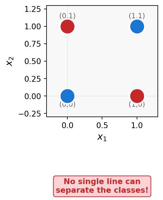
Perceptron Cannot Learn

XOR gate

Non-linearly separable

• The perceptron’s inability to solve XOR was a major limitation identified by Minsky & Papert (1969)
• This led to the first “AI winter” for neural networks
• The solution required multi-layer networks with nonlinear activations

Why XOR breaks the perceptron

The XOR problem: no single line can separate the classes. Red points (output=1) sit on opposite corners.

Solution: Add a hidden layer to create a non-linear decision boundary.

• This is the famous Minsky & Papert (1969) argument that halted neural network research
• XOR requires at least one hidden layer with 2 neurons to solve
• The hidden layer transforms the space so that classes become linearly separable

Backpropagation enabled training of multi-layer networks

• Rumelhart, Hinton, and Williams (1986) introduced error backpropagation
• Uses the chain rule to compute gradients through layers:

\[ \frac{\partial \mathcal{L}}{\partial \theta} = \frac{\partial \mathcal{L}}{\partial \mathbf{a}} \cdot \frac{\partial \mathbf{a}}{\partial \theta} \]

• Allowed training networks with hidden layers, overcoming perceptron limitations

• Backpropagation was actually discovered multiple times (Werbos 1974, others)
• The 1986 paper popularized it and demonstrated its effectiveness
• This breakthrough made deep learning practically possible

Modern architectures build on these foundational principles

• Hierarchical representation learning extracts increasingly abstract features
• Non-linear function approximation enables modeling complex relationships
• Scalability through parallelization and specialized hardware (GPUs, TPUs)

Applications span:

• NLP: machine translation, question answering, text generation
• Vision: object recognition, image segmentation
• Reinforcement learning: game playing, robotics

• Modern transformers, while architecturally different, still rely on the same principles
• Key advances: attention mechanisms, residual connections, layer normalization
• The field continues to evolve rapidly

A neural network is a computational graph of interconnected processing units

• Each neuron computes a weighted sum of inputs plus bias, then applies an activation:

\[ h = f(\mathbf{w}^\top \mathbf{x} + b) \]

• \(\mathbf{w}\): weight vector (learned parameters)
• \(\mathbf{x}\): input vector
• \(b\): bias term
• \(f\): nonlinear activation function

• The biological inspiration is loose—artificial neurons are mathematical abstractions
• The activation function introduces nonlinearity, which is essential for learning complex patterns
• Without nonlinearity, stacking layers would just produce another linear transformation

Networks are organized into layers with distinct roles

Input Layer

x₁

x₂

x₃

→

Hidden Layer(s)

h₁

h₂

→

Output Layer

ŷ₁

ŷ₂

• Input layer: Receives raw features (e.g., word embeddings)
• Hidden layers: Learn intermediate representations
• Output layer: Produces predictions (often via softmax)

• Hidden layers are where the “magic” happens—they learn useful feature representations
• Deeper networks can learn more abstract, hierarchical features
• The number of layers and neurons per layer are hyperparameters to tune

Feedforward networks process information in one direction only

• Data flows from input → hidden → output with no cycles
• Each layer’s output becomes the next layer’s input
• The entire computation is a composition of functions:

\[ \hat{y} = f^{[L]}(f^{[L-1]}(\cdots f^{[1]}(\mathbf{x})\cdots)) \]

• “Feedforward” means no feedback connections—pure function composition
• This is in contrast to recurrent networks, which have cycles
• Feedforward networks are simpler to train and analyze

Recurrent networks can model sequential dependencies through cycles

• Allow information to persist across time steps
• Hidden state \(\mathbf{h}_t\) encodes history of previous inputs
• Essential for language modeling, speech recognition, time series

Feedforward

Fixed-size input → Fixed-size output

Image classification, sentiment analysis

Recurrent

Sequence → Sequence or output

Language modeling, machine translation

• Recurrent networks introduce temporal dynamics and memory
• However, they can be harder to train (vanishing/exploding gradients)
• Modern transformers handle sequences differently, using attention

Neural network computation is fundamentally linear algebra

• Inputs, parameters, and activations are vectors and matrices
• Core operation: matrix-vector multiplication plus bias

\[ \mathbf{z} = \mathbf{W}\mathbf{x} + \mathbf{b} \]

• Dimensions must align: if \(\mathbf{x} \in \mathbb{R}^d\) and \(\mathbf{W} \in \mathbb{R}^{m \times d}\), then \(\mathbf{z} \in \mathbb{R}^m\)

• Getting dimensions right is a common source of bugs
• Think of \(\mathbf{W}\) as learning \(m\) different linear combinations of the \(d\) input features
• Each row of \(\mathbf{W}\) corresponds to one output neuron’s weights

Dot products measure vector similarity

\[ \mathbf{a} \cdot \mathbf{b} = \|\mathbf{a}\| \|\mathbf{b}\| \cos(\theta) \]

Similar (θ ≈ 0°)

→ →

a · b > 0

Vectors point same direction

Orthogonal (θ = 90°)

→ ↑

a · b = 0

Vectors are unrelated

Opposite (θ ≈ 180°)

→ ←

a · b < 0

Vectors point opposite

Neural networks use dot products to measure relevance between vectors

• When embeddings are normalized, dot product equals cosine similarity
• This is fundamental to how attention works in transformers
• Query-key dot products measure “how relevant is this token to that token?”
• Higher dot product = more similar/relevant representations

Matrix multiplication computes all pairwise dot products

• If \(\mathbf{Q} \in \mathbb{R}^{n \times d}\) and \(\mathbf{K} \in \mathbb{R}^{m \times d}\), then:

\[ (\mathbf{Q}\mathbf{K}^\top)_{ij} = \mathbf{q}_i \cdot \mathbf{k}_j \]

Q (3×d)

q₁

q₂

q₃

×

K^T (d×4)

k₁

k₂

k₃

k₄

=

Similarity (3×4)

q₁·k₁

q₁·k₂

q₁·k₃

q₁·k₄

q₂·k₁

q₂·k₂

q₂·k₃

q₂·k₄

q₃·k₁

q₃·k₂

q₃·k₃

q₃·k₄

One matrix multiply computes all 12 similarities in parallel!

• This is exactly what happens in transformer attention: QK^T
• GPUs are optimized for matrix multiplication—extremely fast
• Computing all pairwise similarities enables parallel processing
• Next lecture: these similarity scores become attention weights after softmax

Activation functions introduce essential nonlinearity

After computing \(\mathbf{z}\), we apply an activation function elementwise:

\[ \mathbf{h} = \phi(\mathbf{z}) \]

ReLU

max(0, z)

Simple, fast, sparse

Sigmoid

1/(1+e⁻ᶻ)

Output in (0,1)

Tanh

(eᶻ-e⁻ᶻ)/(eᶻ+e⁻ᶻ)

Output in (-1,1)

• ReLU is the most common choice today—simple and effective
• Sigmoid/tanh can cause vanishing gradients in deep networks
• Without nonlinearity, any stack of linear layers = one linear layer

Activation function shapes determine gradient flow

Activation functions and their gradients. ReLU dominates modern networks due to its constant gradient for positive inputs.

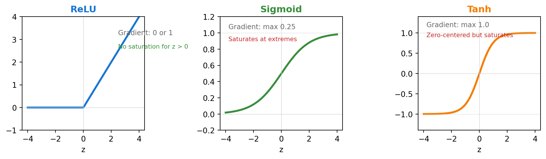
Why ReLU dominates: Constant gradient (1) for positive inputs prevents vanishing gradients in deep networks.

• Sigmoid gradient is at most 0.25—multiplying across layers causes exponential decay
• Tanh is zero-centered (better than sigmoid) but still saturates
• ReLU’s “dead neuron” problem: if z < 0 always, gradient is always 0
• Variants like Leaky ReLU and GELU address the dead neuron issue

The softmax function converts scores to probabilities

• Transforms a vector \(\mathbf{z}\) into a probability distribution:

\[ \operatorname{softmax}(z_i) = \frac{\exp(z_i)}{\sum_{j=1}^d \exp(z_j)} \]

• Guarantees: \(\sum_i \operatorname{softmax}(z_i) = 1\) and \(0 < \operatorname{softmax}(z_i) < 1\)

• The largest logit (3.2) gets most of the probability mass (0.74)
• Softmax is “soft” because it doesn’t hard-select one class
• This is essential for multi-class classification with cross-entropy loss

Part 2: Feedforward Neural Networks

Each layer transforms its input through weights, bias, and activation

For layer \(i\):

\[ \mathbf{x}^{[i]} = f^{[i]}\left( \mathbf{W}^{[i]} \mathbf{x}^{[i-1]} + \mathbf{b}^{[i]} \right) \]

• \(\mathbf{W}^{[i]}\): learnable weight matrix
• \(\mathbf{b}^{[i]}\): learnable bias vector
• \(f^{[i]}\): activation function

x⁽ⁱ⁻¹⁾

→

W⁽ⁱ⁾x + b⁽ⁱ⁾

→

f⁽ⁱ⁾(·)

→

x⁽ⁱ⁾

• This is the fundamental building block—everything else builds on this
• Parameters \(\mathbf{W}\) and \(\mathbf{b}\) are learned during training
• The activation function choice affects learning dynamics significantly

Activation functions serve different purposes in different layers

Location	Common Choice	Purpose
Hidden layers	ReLU, GELU	Introduce nonlinearity, sparse activation
Binary output	Sigmoid	Probability in [0,1]
Multi-class output	Softmax	Probability distribution
Regression output	None (linear)	Unbounded real values

• Softmax is typically only used in the output layer for classification
• ReLU is the default choice for hidden layers in most modern networks
• GELU (Gaussian Error Linear Unit) is popular in transformers

The universal approximation theorem guarantees theoretical expressivity

Theorem: A feedforward network with one hidden layer and sufficient neurons can approximate any continuous function on a compact domain to arbitrary precision.

\[ \forall \epsilon > 0, \exists \hat{f}: \sup_{x \in K} |f(x) - \hat{f}(x)| < \epsilon \]

But this doesn’t mean shallow networks are always practical:

• May require exponentially many neurons
• Says nothing about learnability or generalization

• This is an existence theorem, not a construction
• A single hidden layer might need more neurons than atoms in the universe
• Depth provides more efficient representations for many functions

Depth enables efficient representation of compositional structure

Shallow Network

O(2ⁿ)

neurons for some functions

Deep Network

O(n)

neurons for same functions

• Telgarsky (2016): Some functions require exponentially more units in shallow vs. deep networks
• Depth captures hierarchical/compositional structure naturally
• Language has recursive, hierarchical structure → depth helps

• Think of composing simple operations: deep networks compose naturally
• Image recognition: edges → textures → parts → objects
• Language: characters → morphemes → words → phrases → sentences

Part 3: Learning and Training Algorithms

Supervised learning optimizes parameters using labeled examples

• Training data: pairs \((\mathbf{x}, y)\) of inputs and target outputs
• Model predicts: \(\hat{y} = f_\theta(\mathbf{x})\)
• Objective: minimize average loss over training set

\[ \mathcal{L}(\theta) = \frac{1}{N} \sum_{i=1}^N \ell\big(f_\theta(\mathbf{x}_i), y_i\big) \]

• \(\theta\) represents all learnable parameters (weights and biases)
• The loss function measures how wrong our predictions are
• Minimizing loss (hopefully) improves generalization to new data

Loss functions measure prediction quality

Cross-Entropy (Classification)

ℓ = −Σₖ yₖ log ŷₖ

Penalizes low probability on correct class

MSE (Regression)

ℓ = (y − ŷ)²

Penalizes squared deviation from target

Cross-entropy loss for classification:

\[ \ell_{\text{CE}}(\hat{\mathbf{y}}, \mathbf{y}) = -\sum_{k=1}^K y_k \log \hat{y}_k \]

• Cross-entropy is the standard for classification tasks
• It’s closely related to maximum likelihood estimation
• The choice of loss function should match the task

NLP applications of supervised learning span many tasks

Task	Input \(\mathbf{x}\)	Output \(y\)
POS tagging	Word + context	POS tag (noun, verb, etc.)
Sentiment	Sentence/document	Sentiment class
NER	Word + context	Entity type or O
Text classification	Document	Topic/category

• The framework is general—same learning algorithm, different tasks
• Input representation (embeddings) matters a lot
• Modern approaches often use pre-trained representations

Backpropagation computes gradients efficiently via the chain rule

• We need \(\frac{\partial L}{\partial W^{[l]}}\) for each layer to update weights
• Backprop propagates error signals backward through the network

\[ \frac{\partial L}{\partial W^{[l]}} = \delta^{[l]} (a^{[l-1]})^T \]

where \(\delta^{[l]} = \frac{\partial L}{\partial z^{[l]}}\) is the error signal at layer \(l\).

• Backprop is just efficient application of the chain rule
• “Error signal” tells us how much each neuron contributed to the loss
• This is computed in one backward pass—linear in network size

Error signals propagate backward through the network

Forward Pass

Input x

→

Hidden h¹

→

Hidden h²

→

Output ŷ

Backward Pass

∂L/∂ŷ

←

δ²

←

δ¹

←

∂L/∂x

The recursive error signal computation:

\[ \delta^{[l]} = \left( W^{[l+1]}\right)^T \delta^{[l+1]} \odot \sigma' (z^{[l]}) \]

• \(\odot\) is element-wise multiplication
• \(\sigma'\) is the derivative of the activation function
• This recursion is why it’s called “back” propagation

Gradients drive parameter updates via gradient descent

Weight update rule:

\[ W^{[l]} \leftarrow W^{[l]} - \eta \frac{\partial L}{\partial W^{[l]}} \]

\[ b^{[l]} \leftarrow b^{[l]} - \eta \frac{\partial L}{\partial b^{[l]}} \]

• \(\eta\): learning rate (critical hyperparameter)
• Too high → unstable, may diverge; Too low → slow convergence

• The learning rate is arguably the most important hyperparameter
• Modern practice: use learning rate schedules (warmup, decay)
• Adaptive optimizers (Adam) adjust learning rates per-parameter

Gradient descent navigates the loss landscape

Gradient descent behavior with different learning rates. The learning rate η controls convergence speed and stability.

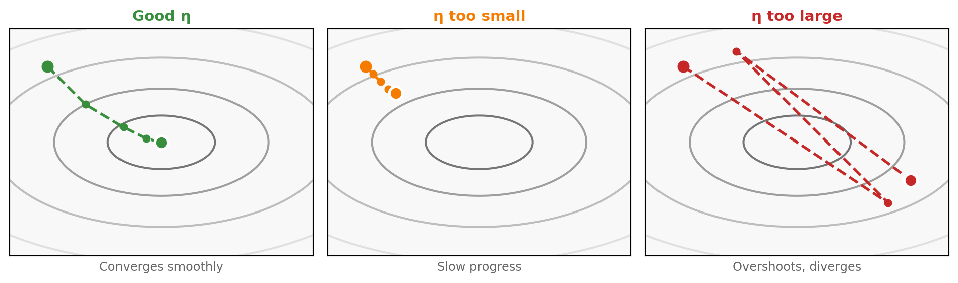
Gradient descent follows the steepest downhill direction; step size η determines how far we move each update.

• The loss landscape shows loss as a function of parameters (here simplified to 2D)
• Contour lines connect points of equal loss; the center is the minimum
• In practice: thousands or millions of dimensions, much more complex topology

Backpropagation is not an optimizer—it computes gradients for optimizers

Common misconception: Backprop = training algorithm

Reality:

• Backprop: efficient gradient computation method
• SGD/Adam/etc.: optimization algorithms that use gradients
• Together they enable training, but they’re distinct concepts

Loss L

→

Backpropagation

→

Gradients ∇L

→

Optimizer
(SGD, Adam)

→

New Weights

• This distinction matters for understanding the literature
• Different optimizers can use the same backprop-computed gradients differently
• Modern frameworks (PyTorch, TensorFlow) separate these cleanly

SGD processes mini-batches for efficient, noisy updates

Stochastic Gradient Descent:

\[ \theta_{t+1} = \theta_t - \eta \nabla_\theta L(\theta_t; \mathcal{B}_t) \]

• \(\mathcal{B}_t\): random mini-batch at step \(t\)
• Noisy gradients can help escape local minima
• Much faster than full-batch gradient descent

• “Stochastic” because we use random samples, not the full dataset
• Typical batch sizes: 32, 64, 128, 256
• Larger batches → more stable gradients, but slower updates

Adam combines momentum and adaptive learning rates

Adam update equations:

\[ m_t = \beta_1 m_{t-1} + (1 - \beta_1) \nabla_\theta L(\theta_t) \]

\[ v_t = \beta_2 v_{t-1} + (1 - \beta_2) (\nabla_\theta L(\theta_t))^2 \]

\[ \theta_{t+1} = \theta_t - \eta \frac{m_t}{\sqrt{v_t} + \epsilon} \]

• \(m_t\): momentum (smoothed gradient)
• \(v_t\): adaptive scaling (per-parameter)
• Default: \(\beta_1=0.9\), \(\beta_2=0.999\), \(\epsilon=10^{-8}\)

• Adam is the default choice for most deep learning tasks
• Adapts learning rate per-parameter based on gradient history
• Generally more robust to hyperparameter choices than SGD
• AdamW variant decouples weight decay from gradient updates—standard for transformers

Optimizers behave differently on complex loss surfaces

Optimizer behavior on a saddle-like loss surface. SGD oscillates, Momentum smooths, Adam adapts step sizes per-parameter.

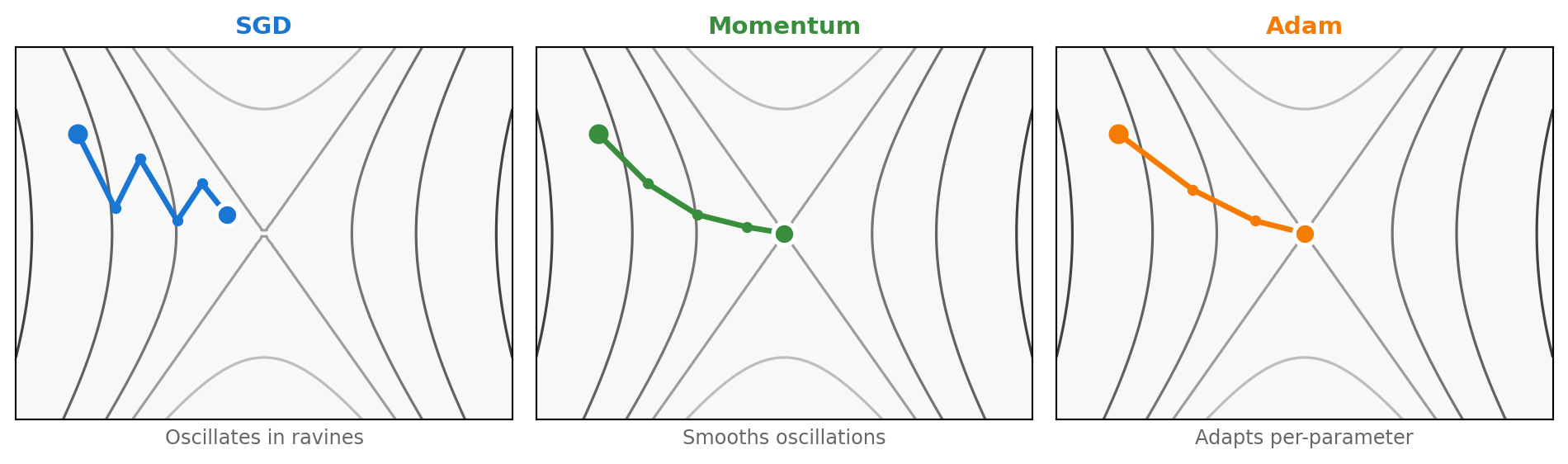
Adam combines momentum’s smoothing with per-parameter learning rate scaling—faster and more robust convergence.

• On saddle points: SGD gets stuck, momentum helps escape, Adam adapts step sizes
• Adam’s adaptive scaling means it can take larger steps in flat directions, smaller in steep ones
• For transformers: AdamW (with decoupled weight decay) is standard

Regularization prevents overfitting by constraining model capacity

L2 Regularization

L' = L + λ‖θ‖²

Penalizes large weights

Dropout

hᵢ = rᵢ · hᵢ

rᵢ ~ Bernoulli(p)

Early Stopping

Stop when val↑

Monitor validation loss

• L2 regularization (weight decay) shrinks weights toward zero
• Dropout randomly “turns off” neurons during training
• Early stopping prevents training too long on the training set
• Modern transformers typically use AdamW with weight decay around 0.01–0.1, layer normalization, and little to no dropout

Dropout forces the network to learn redundant representations

• During training: randomly set fraction \(p\) of activations to 0
• During inference: use all neurons, scale by \((1-p)\)
• Effect: no single neuron can become too important

Training (with dropout)

→

→

Some neurons "dropped"

Inference (no dropout)

→

→

All neurons active

• Dropout can be seen as training an ensemble of subnetworks
• Typical dropout rates: 0.1-0.5 depending on layer
• Usually not applied to input layer or output layer
• In transformers, dropout is often minimal or absent in attention/FFN layers; weight decay does most of the regularization work

Dropout signficantly reduces overfitting

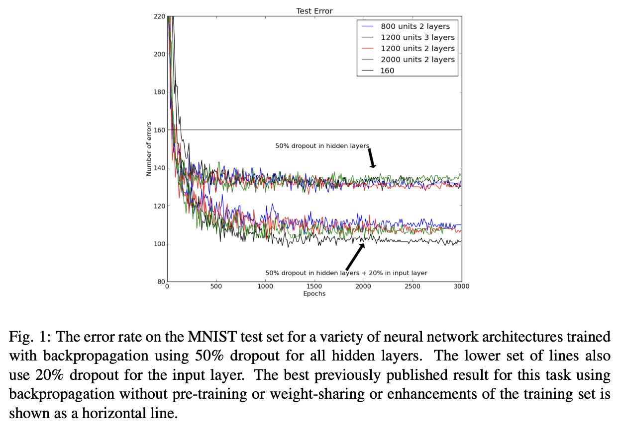
Improving neural networks by preventing co-adaptation of feature detectors (Hinton et al., 2012)

• Results on MNIST with 50% dropout in hidden layers
• Improvement is consistent across different network sizes (800–8000 units) and depths (2–3 layers)
• Adding 20% dropout to input layer provides additional benefit

Part 4: Advanced Architectures and Extensions

Vanishing gradients make training deep networks difficult

• Gradients shrink exponentially when propagated through many layers
• For sigmoid: \(\sigma'(z) \leq 0.25\), so gradient decays by at least 4× per layer

\[ \delta^{[l]} = (W^{[l+1]})^T \delta^{[l+1]} \odot \sigma'(z^{[l]}) \]

• With 10 layers: gradient shrinks by \(\approx 4^{10} \approx 10^6\)

• This is why deep networks were hard to train before ~2012
• Early layers barely learn because their gradients are tiny
• Solutions: ReLU activation, careful initialization, residual connections
• Hochreiter (1991) formally analyzed this vanishing gradient problem

Exploding gradients cause training instability

• The opposite problem: gradients grow exponentially
• Occurs when \(\|W^{[l]}\| > 1\) and compounds across layers
• Symptoms: NaN losses, weights becoming infinite

Solutions:

• Gradient clipping: \(g \leftarrow g \cdot \frac{\tau}{\|g\|}\) if \(\|g\| > \tau\)
• Careful weight initialization
• Batch normalization

• Gradient clipping is essential for training RNNs
• The threshold τ is typically 1.0 or 5.0
• Modern architectures are designed to avoid this problem

Proper initialization maintains gradient flow

Xavier/Glorot initialization:

\[ \text{Var}[W_{ij}] = \frac{2}{n_{in} + n_{out}} \]

He initialization (for ReLU):

\[ \text{Var}[W_{ij}] = \frac{2}{n_{in}} \]

• Goal: keep activation and gradient variance stable across layers
• Critical for training networks with 10+ layers

• Before proper initialization, deep networks simply wouldn’t train
• He initialization accounts for ReLU killing half the activations
• Modern frameworks use these by default

Residual connections enable training of very deep networks

• Key idea: Add input directly to output via “skip connection”

\[ \mathbf{h}^{[l+1]} = f(\mathbf{h}^{[l]}) + \mathbf{h}^{[l]} \]

h⁽ˡ⁾

↓

f(·)

↓

skip

+

→

h⁽ˡ⁺¹⁾

Why it helps: Gradient flows directly through the skip connection:

\[ \frac{\partial \mathbf{h}^{[l+1]}}{\partial \mathbf{h}^{[l]}} = \frac{\partial f}{\partial \mathbf{h}^{[l]}} + \mathbf{I} \]

• The identity term I ensures gradient doesn’t vanish even if ∂f/∂h is small
• Introduced by He et al. (2015) for image recognition (ResNets)
• Critical for training networks with 100+ layers
• Transformers use residual connections after every sublayer (attention + FFN)

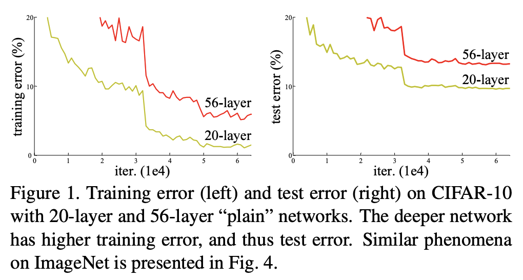
Residual connections: empirical evidence

Training error on CIFAR-10: without residuals, a 56-layer “plain” network performs worse than a 20-layer network—even on training data. With residual connections (right), deeper networks consistently outperform shallower ones.

• This is NOT overfitting—deeper plain networks have higher training error too
• The degradation problem shows optimization difficulty, not capacity issues
• Residual connections solve this by providing gradient highways

Figure from He et al. (2015), “Deep Residual Learning for Image Recognition”

Layer normalization stabilizes training of deep networks

\[ \text{LayerNorm}(\mathbf{x}) = \gamma \odot \frac{\mathbf{x} - \mu}{\sigma + \epsilon} + \beta \]

• \(\mu, \sigma\): mean and std computed across features (per example)
• \(\gamma, \beta\): learnable scale and shift parameters

Batch Normalization

Normalize across batch dimension

• Depends on batch statistics
• Different behavior train vs test
• Problematic for variable-length sequences

Layer Normalization

Normalize across feature dimension

• Independent of batch size
• Same behavior train and test
• Works with any sequence length ✓

• Layer norm is the standard choice for transformers and RNNs
• Applied after residual connection: LayerNorm(x + Sublayer(x))
• Stabilizes activations, allowing larger learning rates
• Next lecture: transformers apply layer norm after every attention and FFN sublayer

Comparing normalization techniques: BatchNorm vs LayerNorm vs RMSNorm

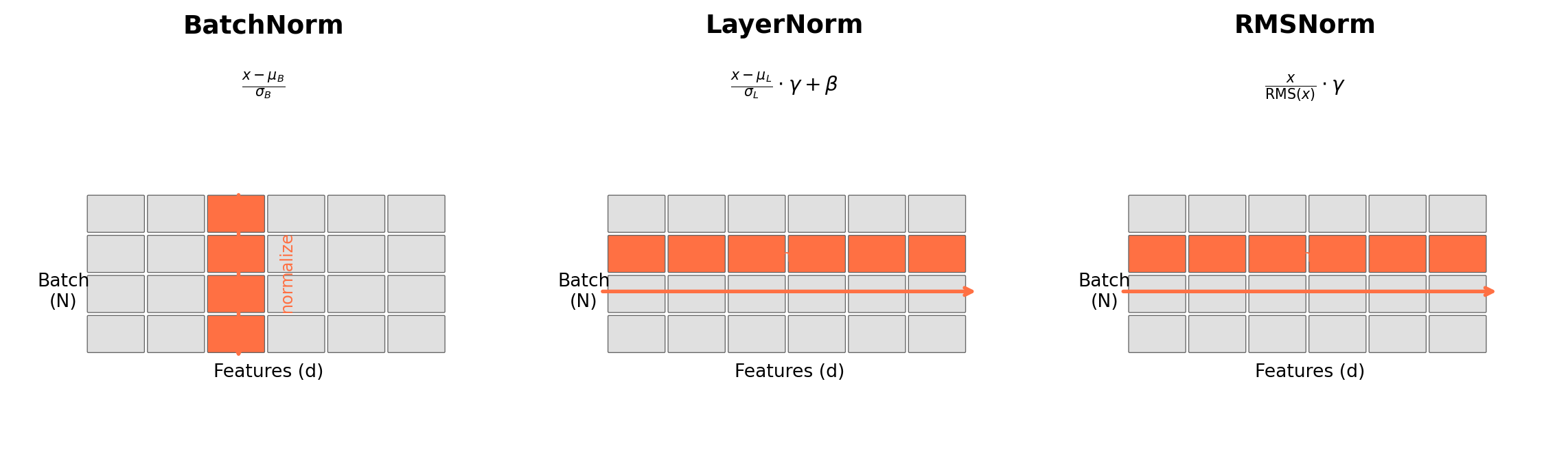
	BatchNorm	LayerNorm	RMSNorm
Normalizes	Batch dim	Feature dim	Feature dim
Train/Test	Different	Same	Same
Used in	CNNs	Transformers	LLaMA, Gemma

• BatchNorm normalizes across the batch: requires batch statistics, different behavior at train vs test time
• LayerNorm normalizes across features: batch-independent, consistent train/test behavior
• RMSNorm removes mean-centering from LayerNorm: \(\text{RMS}(x) = \sqrt{\frac{1}{d}\sum_i x_i^2}\)
• RMSNorm is ~10-15% faster than LayerNorm with similar empirical performance
• Modern LLMs (LLaMA, Gemma, Mistral) prefer RMSNorm for efficiency
• Trade-off: slightly less expressive (no learned bias) but faster computation

RNNs model sequences by maintaining state across time steps

\[ \mathbf{h}_t = f(\mathbf{W}_{xh} \mathbf{x}_t + \mathbf{W}_{hh} \mathbf{h}_{t-1} + \mathbf{b}_h) \]

h₁

↑

x₁

→

h₂

↑

x₂

→

h₃

↑

x₃

→

h₄

↑

x₄

→

ŷ

• Hidden state \(\mathbf{h}_t\) encodes information from \(x_1, \ldots, x_t\)
• Same parameters (\(\mathbf{W}_{xh}, \mathbf{W}_{hh}\)) used at every time step

• The hidden state acts as “memory” of past inputs
• Parameter sharing across time is a key inductive bias
• Enables processing sequences of any length

The RNN sequential bottleneck limits parallelization

• \(\mathbf{h}_t\) depends on \(\mathbf{h}_{t-1}\) creates a dependency chain
• Cannot compute \(\mathbf{h}_5\) until \(\mathbf{h}_1, \mathbf{h}_2, \mathbf{h}_3, \mathbf{h}_4\) are finished

h₁

WAIT

→

h₂

WAIT

→

h₃

WAIT

→

h₄

WAIT

→

h₅

O(T) sequential steps for sequence length T

Implications:

• Cannot fully utilize parallel hardware (GPUs have thousands of cores)
• Training time scales linearly with sequence length
• Key question: What if we could process all tokens at once?

• This sequential bottleneck is a fundamental limitation of RNNs
• GPUs are designed for parallel computation—RNNs can’t exploit this fully
• Transformers solve this by removing the sequential dependency entirely
• Next lecture: attention allows O(1) depth for any sequence length

Autoregressive vs bidirectional processing

Autoregressive (left-to-right): Each position only sees the past

\[ P(x_1, x_2, \ldots, x_n) = \prod_{t=1}^{n} P(x_t | x_1, \ldots, x_{t-1}) \]

Bidirectional: Each position sees the entire sequence

Autoregressive (GPT)

The

cat

sat

?

?

Position 3 sees only positions 1-2

Bidirectional (BERT)

The

cat

[MASK]

on

mat

Position 3 sees all positions

• Autoregressive models are used for generation (predict next token)
• Bidirectional models are used for understanding (classify, extract)
• In transformers: autoregressive = causal masking (can’t look ahead)
• BERT uses bidirectional attention; GPT uses causal (autoregressive) attention

Standard RNNs struggle with long-range dependencies

"The cat, which was sitting on the mat in the living room where my grandmother used to read her favorite novels during the winter evenings, was hungry."

The verb "was" must agree with "cat" despite 20+ intervening words.

• Gradient signal degrades over long distances
• LSTM and GRU use gating mechanisms to preserve information
• Transformers use attention to directly connect distant positions

• This is a fundamental limitation of vanilla RNNs
• LSTM adds cell state with additive updates (better gradient flow)
• Transformers avoid the sequential bottleneck entirely

Context as a weighted combination of representations

• What if we could directly access all previous representations?
• Key insight: compute a weighted sum based on relevance

\[ \text{output}_t = \sum_{j=1}^{t} \alpha_{tj} \cdot \mathbf{v}_j \]

• \(\alpha_{tj}\): attention weight (how relevant is position \(j\) to position \(t\)?)
• \(\mathbf{v}_j\): value vector at position \(j\)

v₁

α₄₁ = 0.1

v₂

α₄₂ = 0.5

v₃

α₄₃ = 0.3

→

output₄

Σ αᵢ · vᵢ

• This is the core idea behind attention mechanisms
• Attention weights \(\alpha\) are computed from how “relevant” each position is
• In transformers: relevance is measured by dot product similarity (q · k)
• This removes the sequential bottleneck—all positions accessed directly

Attention weights reveal what the model focuses on

Attention from "it" in: "The cat sat on the mat because it was tired"

The

cat

sat

on

the

mat

because

it

was

it →

0.05

0.45

0.10

0.03

0.02

0.15

0.05

0.10

0.05

What attention reveals:

The pronoun "it" attends most strongly to "cat" (0.45)—the model has learned coreference!

Darker = higher attention weight

• This is a simplified example; real attention patterns are learned, not hand-coded
• Different attention heads learn different relationships (syntax, coreference, etc.)
• Attention provides some interpretability—we can see what the model “looks at”

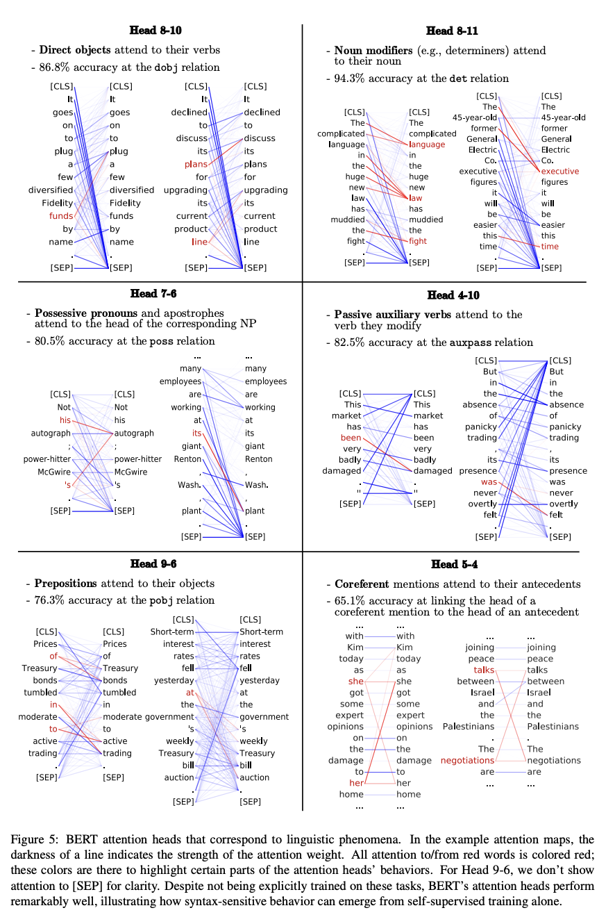
BERT attention learns coreference resolution

Attention patterns from BERT showing coreference resolution. The model learns to link pronouns to their antecedents—here “it” attends strongly to “cat” and “dog” to resolve what each pronoun refers to.

• Different attention heads specialize in different linguistic relationships
• Some heads track syntax (subject-verb), others track coreference (pronoun-antecedent)
• This emergent behavior arises from pretraining—not explicitly supervised

Figure from Clark et al. (2019), “What Does BERT Look At? An Analysis of BERT’s Attention”

Position information must be explicitly encoded

• Without recurrence, order information is lost
• “Dog bit man” and “man bit dog” would be identical!

Without Position Info

{dog, bit, man} = {man, bit, dog}

Bag of words—order lost!

With Position Encoding

(dog, 1), (bit, 2), (man, 3)

Order preserved via position

Key question: How do we inject position information into parallel architectures?

• RNNs encode position implicitly through sequential processing
• Parallel architectures (transformers) need explicit position encodings
• Next lecture: sinusoidal and learned positional encodings
• This is why transformers add position embeddings to token embeddings

Sinusoidal position encodings (Vaswani et al., 2017)

Add a position-dependent vector to each token embedding:

\[ PE_{(pos, 2i)} = \sin\left(\frac{pos}{10000^{2i/d}}\right) \quad PE_{(pos, 2i+1)} = \cos\left(\frac{pos}{10000^{2i/d}}\right) \]

Sinusoidal position encodings: each position gets a unique pattern. Low dimensions oscillate rapidly (fine position), high dimensions oscillate slowly (coarse position).

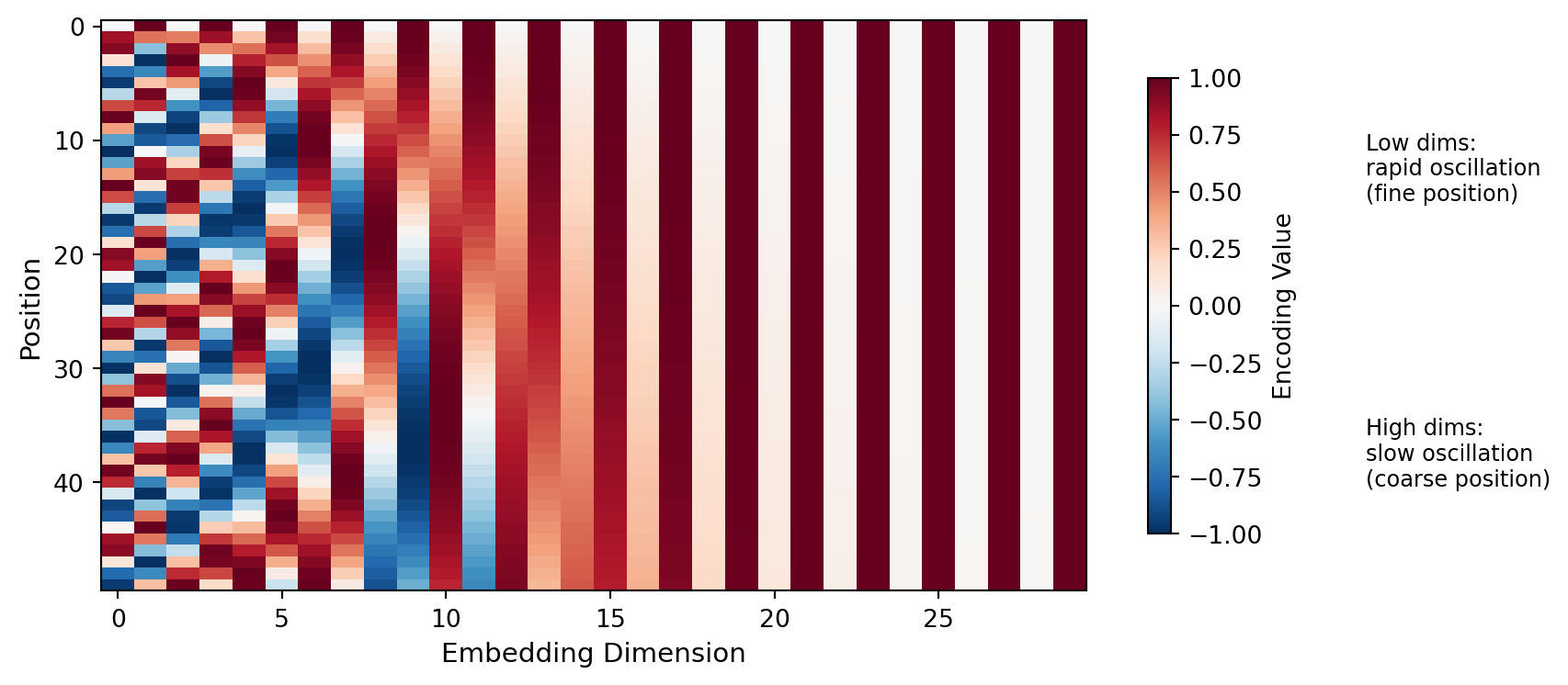
Key properties: Each position gets a unique encoding; relative positions computable via linear transformation; generalizes to longer sequences.

• Low dimensions (left) oscillate rapidly—encode fine position differences
• High dimensions (right) oscillate slowly—encode coarse position
• Modern models often use learned position embeddings instead, but sinusoidal is still common

Part 5: Applications

Neural networks power core NLP tasks

Task	Architecture	Output
Text classification	Feedforward / CNN / Transformer	Class probabilities (softmax)
Language modeling	RNN / Transformer	Next token probabilities
Sequence labeling	BiLSTM / Transformer	Tag per token
Machine translation	Encoder-decoder	Target sequence

• Softmax appears everywhere—it’s the standard output for classification
• Language modeling is foundational—it underlies GPT, BERT pretraining
• Modern systems typically use transformers for all these tasks

Text classification assigns labels to documents

Document
'Great movie!'

→

Embedding
Layer

→

Encoder
(CNN/LSTM/Transformer)

→

Pooling

→

Dense

→

Softmax

→

P(pos)=0.92
P(neg)=0.08

Applications: Sentiment analysis, spam detection, topic classification

• Pooling aggregates variable-length text into fixed-size representation
• Common pooling: mean, max, or [CLS] token in transformers
• Pre-trained models (BERT) dramatically improved text classification

Language modeling predicts the next token in a sequence

\[ P(w_t | w_1, \ldots, w_{t-1}) = \text{softmax}(\mathbf{W} \mathbf{h}_{t-1} + \mathbf{b}) \]

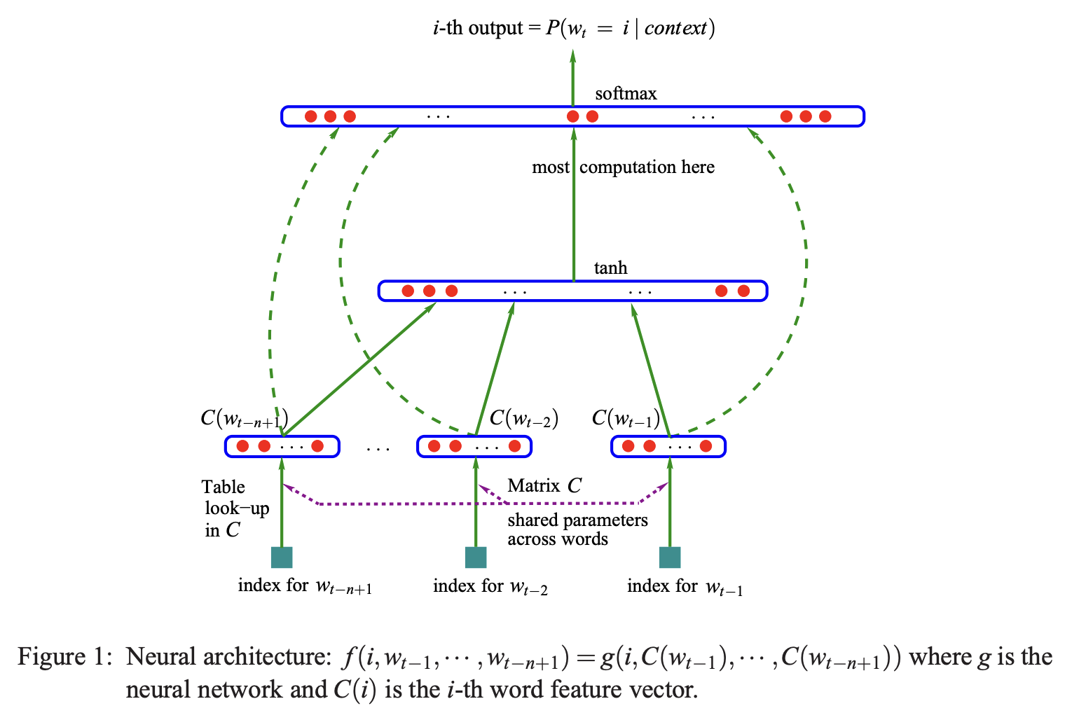
Bengio et al. (2003) neural language model: word embeddings → hidden layer → softmax over vocabulary

• Language modeling is perhaps the most important NLP task today
• GPT models are essentially very large language models
• The “pre-train then fine-tune” paradigm revolutionized NLP
• Bengio’s 2003 paper introduced the idea of learning word embeddings jointly with the LM

Neural networks excel across diverse domains

Computer Vision

CNNs for image classification, object detection, segmentation

Reinforcement Learning

Deep Q-networks, policy gradients for game playing, robotics

Bioinformatics

Protein structure prediction (AlphaFold), genomics

Recommendations

Neural collaborative filtering, content-based systems

• Same fundamental principles (backprop, gradient descent) apply
• Architecture choices encode domain-specific inductive biases

• CNNs encode translation invariance for images
• Graph neural networks encode relational structure
• The core learning algorithms are remarkably general

Part 6: Further Reading and Historical Notes

Key references for deeper understanding

Textbooks:

• Goodfellow, Bengio, & Courville (2016), Deep Learning — comprehensive theory and practice
• Jurafsky & Martin, Speech and Language Processing Ch. 6-8

• The Goodfellow textbook is freely available online
• Original papers provide important historical context

Key milestones in neural network history

Foundations

1943 — McCulloch-Pitts neuron

1958 — Perceptron (Rosenblatt)

1969 — Perceptrons book → AI Winter

Revival

1986 — Backpropagation

1990 — Elman RNNs

1997 — LSTM (Hochreiter & Schmidhuber)

Modern Era

2012 — AlexNet → Deep learning revolution

2017 — Transformer architecture

2018 — BERT, GPT

• Multiple “AI winters” when progress stalled
• Key enablers: compute (GPUs), data (internet), algorithms (backprop, attention)
• We’re currently in a period of rapid advancement

Summary: Neural Networks - Key Takeaways

• Architecture: Networks of neurons organized in layers; feedforward vs. recurrent
• Learning: Supervised learning minimizes loss via gradient descent
• Backpropagation: Efficient gradient computation using the chain rule
• Optimization: SGD, Adam; regularization (dropout, L2) prevents overfitting
• Challenges: Vanishing/exploding gradients addressed by careful design
• Applications: Text classification, language modeling, and beyond

• These fundamentals underpin all modern NLP systems
• Next lectures: embeddings, transformers, large language models
• Recommend reviewing the math if it’s unfamiliar

Questions?

Coming up next: Transformers and attention mechanisms

Resources:

• Goodfellow et al. Deep Learning (free online)
• 3Blue1Brown neural network videos (visual intuition)
• PyTorch tutorials (hands-on practice)