Text Classification

Rob Minneker

2026-01-15

Administrivia

• Course website has some updates (for real)
• A1 is released! Due the 29th, read it and plan ahead

Sources

Content derived from: J&M Ch. 4

Google Cloud Education Credits

• Google has graciously given our course cloud credits!
• $50 per student to use this quarter
• Instructions on how to redeem on Ed

Evaluation metrics like accuracy, precision, recall, and F1-score measure classifier performance. (1/8)

• Evaluation metrics like accuracy, precision, recall, and F1-score measure classifier performance.

• Accuracy quantifies overall correctness:

\[ \text{Accuracy} = \frac{TP + TN}{TP + FP + TN + FN} \]

where \(TP\) = true positives, \(TN\) = true negatives, \(FP\) = false positives, \(FN\) = false negatives.

Optional discussion question: - Highlight the confusion matrix as the foundation for understanding how these metrics relate to classifier successes and errors.

Spam dataset: Is this a good model?

• Suppose 1,000,000 emails: 999,000 ham (99.9%) and 1,000 spam (0.1%).
• A model predicts ham for every message.
• Accuracy = 999,000 / 1,000,000 = 99.9%.
• Is this a good model?

• This classifier misses all spam, but accuracy alone hides the failure.

Evaluation metrics like accuracy, precision, recall, and F1-score measure classifier performance. (2/8)

• Precision and recall are class-specific:

\[ \text{Precision} = \frac{TP}{TP + FP} \qquad \text{Recall} = \frac{TP}{TP + FN} \]

• Precision: proportion of predicted positives that are correct.
• Recall: proportion of actual positives that are retrieved.

• Address the common misconception that accuracy alone is sufficient—explain how it can be misleading for imbalanced datasets.

Evaluation metrics like accuracy, precision, recall, and F1-score measure classifier performance. (3/8)

• F1-score balances precision and recall:

\[ F_1 = 2 \cdot \frac{\text{Precision} \cdot \text{Recall}}{\text{Precision} + \text{Recall}} \]

• Generalizes to \(F_\beta\) for weighting recall vs. precision.

Note

\(F_\beta\) formula: \[ F_\beta = (1 + \beta^2) \cdot \frac{\text{Precision} \cdot \text{Recall}}{(\beta^2 \cdot \text{Precision}) + \text{Recall}} \]

• Stress the importance of choosing evaluation metrics based on the specific application, especially when positive/negative classes are imbalanced or have different risks.

Evaluation metrics like accuracy, precision, recall, and F1-score measure classifier performance. (4/8)

• The confusion matrix summarizes true/false positives/negatives; F1 balances precision and recall.

• The confusion matrix structure:

\[ \begin{array}{c|cc} & \text{Predicted } + & \text{Predicted } - \\ \hline \text{Actual } + & TP & FN \\ \text{Actual } - & FP & TN \\ \end{array} \]

• Clarify the tradeoff between precision and recall, and how the F1-score balances them—use examples like spam detection or disease diagnosis to illustrate.

Evaluation metrics like accuracy, precision, recall, and F1-score measure classifier performance. (5/8)

• Mention that robust evaluation requires proper cross-validation strategies, such as stratified k-fold, to ensure fair metric estimation.

Evaluation metrics like accuracy, precision, recall, and F1-score measure classifier performance. (6/8)

• Directly visualizes classifier errors and successes.
  • Precision-Recall tradeoff:
    • High precision, low recall: conservative classifier.
    • High recall, low precision: aggressive classifier.
    • \(F_1\)-score is harmonic mean, punishing extreme imbalance between precision and recall.

• Transition: Next, we’ll see how these metrics inform model selection and tuning in practical text classification scenarios.

Evaluation metrics like accuracy, precision, recall, and F1-score measure classifier performance. (7/8)

• Choosing the right metric is crucial, especially for imbalanced data and model comparison.

• When would you tolerate more false positives to catch almost every true case (prioritize recall)?

• When would you tolerate more misses to avoid false alarms (prioritize precision)?

• In what situations might you prioritize recall over precision, or vice versa?

Evaluation metrics like accuracy, precision, recall, and F1-score measure classifier performance. (8/8)

• Accuracy can be misleading for imbalanced classes (e.g., rare disease detection).
  • Example: 99% accuracy if classifier always predicts majority class.
  • For skewed data, prefer precision, recall, or \(F_\beta\) tailored to application risk.
  • E.g., spam detection: high recall, moderate precision.
  • Cross-validation strategies (e.g., stratified \(k\)-fold) provide robust estimates and control for class imbalance during evaluation.

Picking \(F_\beta\): example scenarios

• Choose \(F_{\beta=2}\) when recall matters more than precision (misses are costly).
  • Example: cancer screening triage; missing a true case is worse than a false alarm.
  • Example: safety incident detection; you want to catch nearly all real incidents.
• Choose \(F_{\beta=1/2}\) when precision matters more than recall (false alarms are costly).
  • Example: automated legal holds; false positives are expensive to review.
  • Example: account freeze alerts; avoid disrupting legitimate users.

Part 2: Logistic Regression

Discriminative models directly model P(y|x), focusing on decision boundaries between classes. (1/4)

• Discriminative models directly estimate conditional probability \(P(y|x)\), emphasizing decision boundaries.
  • The model focuses on learning the mapping from features \(x\) to labels \(y\), rather than modeling \(P(x)\) or \(P(x, y)\).
  • Contrasts with generative models, which require explicit modeling of the joint distribution \(P(x, y)\) or the marginal \(P(x)\).
  • Inductive bias is centered on maximizing separation between classes in feature space.

Optional discussion question: - Clarify the distinction: discriminative models (e.g., logistic regression) vs. generative models (e.g., Naive Bayes)—the former do not require modeling \(P(x)\) or \(P(x, y)\). - Highlight that logistic regression uses a sigmoid function to map weighted feature sums to probabilities, with parameters learned by minimizing cross-entropy loss.

Discriminative models directly model P(y|x), focusing on decision boundaries between classes. (2/4)

• Logistic regression leverages feature vectors \(x\) and weight parameters \(w\) to model \(P(y=1|x)\) via the sigmoid activation.
  • The model computes:

\[ P(y=1|x) = \sigma(w \cdot x + b) = \frac{1}{1 + e^{-(w \cdot x + b)}} \]

• Point out that the decision boundary is a learned hyperplane, and the model is optimized to maximize separation between classes in feature space.
• Address common misconception: logistic regression does not “regress” in the traditional sense; it’s used for classification, not predicting continuous values.

Logistic regression computes a weighted sum (logit) and applies a sigmoid.

%%{init: {'theme': 'base', 'themeVariables': {'lineColor': '#2f2f2f', 'textColor': '#111111', 'primaryBorderColor': '#2f2f2f', 'fontSize': '18px'}}}%%
flowchart LR
  X["$$x = [x_1, x_2, x_3]$$"]
  W["$$w = [w_1, w_2, w_3]$$"]
  B["$$b$$"]
  Z["$$z = w^\\top x + b$$"]
  S["$$\\hat{y} = \\sigma(z)$$"]
  P["$$P(y=1\\mid x)=\\hat{y}$$"]

  X --> Z
  W --> Z
  B --> Z
  Z --> S --> P

  classDef input fill:#e9f2ff,stroke:#1f4e79,stroke-width:1.2px,color:#0b1f33;
  classDef compute fill:#f3f7ff,stroke:#1f4e79,stroke-width:1.2px,color:#0b1f33;
  classDef output fill:#fff1e6,stroke:#8a3b12,stroke-width:1.2px,color:#3b1a06;
  class X,W,B input;
  class Z,S compute;
  class P output;

• Walk through how each feature is scaled by its weight, summed with a bias to form the logit, then mapped to a probability via the sigmoid.

Discriminative models directly model P(y|x), focusing on decision boundaries between classes. (3/4)

• Training involves optimizing weights \(w\) and bias \(b\) to minimize the cross-entropy loss:

\[ \mathcal{L}(w, b) = -[y \log \hat{y} + (1 - y) \log(1 - \hat{y})] \]

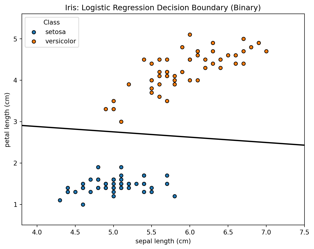
• The decision boundary is the hyperplane \(w \cdot x + b = 0\), learned directly from labeled data.

• Discuss the value of targeted feature engineering in text classification, giving examples like n-grams, TF-IDF, and polarity lexicons.
• Transition: Preview that next, we’ll compare logistic regression with generative approaches and explore their respective strengths and weaknesses in text classification tasks.

Logistic loss is the negative log-likelihood of a Bernoulli model. (1/1)

• Assume \(y^{(i)} \in \{0,1\}\) with Bernoulli likelihood:

\[ p_\theta(y^{(i)} \mid x^{(i)}) = \hat{y}^{(i) y^{(i)}} (1-\hat{y}^{(i)})^{1-y^{(i)}}, \quad \hat{y}^{(i)}=\sigma(w^\top x^{(i)}+b) \]

• MLE maximizes \(\prod_i p_\theta(y^{(i)} \mid x^{(i)})\), equivalently minimizes negative log-likelihood:

\[ -\sum_{i=1}^N \log p_\theta(y^{(i)} \mid x^{(i)}) = -\sum_{i=1}^N \left[y^{(i)} \log \hat{y}^{(i)} + (1-y^{(i)}) \log(1-\hat{y}^{(i)})\right] \]

• This is exactly the binary cross-entropy (logistic) loss.

• Emphasize the equivalence between maximizing likelihood under a Bernoulli model and minimizing cross-entropy.

Iris dataset: binary classification

Classic Iris measurements (sepal/petal lengths) with logistic regression classifying setosa vs. versicolor using a 2D decision boundary.

Discriminative models directly model P(y|x), focusing on decision boundaries between classes. (4/4)

• Discriminative approaches enable robust text classification by allowing targeted feature engineering and direct optimization for accuracy.
  • Feature engineering can encode linguistic, lexical, or syntactic cues (e.g., word presence, n-grams, TF-IDF scores).
  • Empirical performance improves as features are tailored to the structure and nuances of text data.
  • Example: In sentiment classification, features such as polarity lexicon counts or phrase patterns can be incorporated to improve \(P(y|x)\) estimation.

• In what situations might a generative model be preferable to a discriminative model for text classification?

Binary logistic regression models the probability of a binary outcome using the sigmoid function. (1/7)

• Binary logistic regression models the probability of a binary outcome using the sigmoid function.

• For input \(\mathbf{x} \in \mathbb{R}^d\), the model defines the probability of class \(y \in \{0,1\}\) as:

\[ P(y=1|\mathbf{x}; \mathbf{w}, b) = \sigma(\mathbf{w}^\top \mathbf{x} + b) \]

where \(\sigma(z) = \frac{1}{1 + e^{-z}}\) is the sigmoid activation.

• The model parameters are learned by minimizing cross-entropy loss, typically using (stochastic) gradient descent.

Binary logistic regression models the probability of a binary outcome using the sigmoid function. (2/7)

• Intuition: The sigmoid maps real-valued scores to \([0,1]\), enabling probabilistic interpretation for binary classification.

Applications:

• Text sentiment classification (positive/negative)

• Spam detection (spam/not spam)

• Medical diagnosis (disease/no disease)

• Emphasize that outputs are probabilistic, not hard classifications—this allows for confidence estimation in predictions.

Binary logistic regression models the probability of a binary outcome using the sigmoid function. (3/7)

• The model uses cross-entropy loss and optimizes parameters via (stochastic) gradient descent.

• The cross-entropy loss for a single data point is:

\[ \mathcal{L}(\mathbf{w}, b) = -y \log \hat{y} - (1-y) \log (1-\hat{y}) \]

where \(\hat{y} = \sigma(\mathbf{w}^\top \mathbf{x} + b)\).

• For dataset \(\{(\mathbf{x}^{(i)}, y^{(i)})\}_{i=1}^N\), the total loss:

\[ \mathcal{J}(\mathbf{w}, b) = \frac{1}{N} \sum_{i=1}^N \mathcal{L}^{(i)} \]

• Common misconception: logistic regression is not just a linear classifier; the sigmoid enables a probabilistic interpretation.

Binary logistic regression models the probability of a binary outcome using the sigmoid function. (4/7)

Gradient Descent Algorithm:

• For each data point, compute the predicted probability \(\hat{y}\) using the sigmoid function.

• Calculate gradients:

  • \(\nabla_{\mathbf{w}} = (\hat{y} - y) \mathbf{x}\)
  • \(\nabla_b = (\hat{y} - y)\)

• Update parameters:

  • \(\mathbf{w} \leftarrow \mathbf{w} - \eta \nabla_{\mathbf{w}}\)
  • \(b \leftarrow b - \eta \nabla_b\)

• Another misconception: logistic regression is for regression tasks—clarify that despite the name, it is used for classification.

Binary logistic regression models the probability of a binary outcome using the sigmoid function. (5/7)

• Overfitting is a risk, especially with many features; regularization (to be discussed next) is essential to control model complexity.

Binary logistic regression models the probability of a binary outcome using the sigmoid function. (6/7)

• Stochastic gradient descent (SGD) updates parameters using individual samples, improving convergence on large datasets.

• This enables effective classification and sets the stage for regularization to prevent overfitting.

• Logistic regression provides probabilistic outputs, interpretable coefficients, and a convex loss surface, facilitating robust training.

• Overfitting can occur, especially with high-dimensional data; regularization (e.g., L1, L2 penalties) mitigates this by constraining parameter magnitudes.

• Transition: Next, we’ll see how regularization strategies like L1 and L2 penalties help improve generalization and prevent overfitting.

Binary logistic regression models the probability of a binary outcome using the sigmoid function. (7/7)

Next:

• We will examine regularization strategies and their effect on generalization in logistic regression.

Regularization penalties prevent overfitting by constraining parameter magnitudes. (1/3)

• Regularization adds a penalty term to the loss function to discourage large parameter values.
  • \(L_p\) norm: \(\|\mathbf{w}\|_p = \left(\sum_{j=1}^d |w_j|^p\right)^{1/p}\)
  • \(L_1\) regularization (Lasso): \(\|\mathbf{w}\|_1 = \sum_{j=1}^d |w_j|\)
  • \(L_2\) regularization (Ridge): \(\|\mathbf{w}\|_2^2 = \sum_{j=1}^d w_j^2\)
• Regularized loss: \[ \mathcal{J}_{\text{reg}}(\mathbf{w}, b) = \frac{1}{N} \sum_{i=1}^N \mathcal{L}^{(i)} + \lambda \|\mathbf{w}\|_p \]

where \(\lambda\) controls the regularization strength.

• Explain the difference between L1 and L2: L1 encourages sparsity (many weights become zero), while L2 distributes penalty uniformly across weights.

Regularization penalties prevent overfitting by constraining parameter magnitudes. (2/3)

• L2 regularization derives from a Gaussian prior on weights:
  • Prior: \(p(\mathbf{w}) \propto \exp\left(-\frac{\lambda}{2}\|\mathbf{w}\|_2^2\right)\)
  • MAP estimation adds the penalty \(\lambda \|\mathbf{w}\|_2^2\) to the loss.
• L1 regularization derives from a Laplace (double exponential) prior:
  • Prior: \(p(\mathbf{w}) \propto \exp\left(-\lambda \|\mathbf{w}\|_1\right)\)
  • MAP estimation adds the penalty \(\lambda \|\mathbf{w}\|_1\) to the loss.

• Clarify the connection between Bayesian priors and regularization penalties: maximizing posterior probability is equivalent to minimizing regularized loss.

Regularization penalties prevent overfitting by constraining parameter magnitudes. (3/3)

• L1 regularization promotes sparsity by setting many weights to zero, enabling feature selection.

• L2 regularization shrinks weights uniformly, improving generalization without feature selection.

• Practical guidance:

  • Use L2 (Ridge) for dense feature spaces or when all features may be informative.
  • Use L1 (Lasso) when feature selection is desired or the feature space is sparse.
  • Elastic Net combines L1 and L2 for balanced regularization.

• (Discussion) When might you prefer L1 over L2, or vice versa, in text classification applications?

• Discussion question: Why might we prefer probabilistic outputs over hard class labels in some applications?

Multiclass logistic regression can be done via one-vs-rest or softmax approaches. (1/3)

• Multiclass logistic regression can be performed using either one-vs-rest or softmax approaches.
  • In the one-vs-rest (OvR) strategy, \(K\) binary classifiers are trained, one per class, each distinguishing one class from all others.
  • For class \(k\), the classifier computes \(P(y = k \mid \mathbf{x}) = \sigma(\mathbf{w}_k^\top \mathbf{x} + b_k)\)
  • The predicted class is \(\arg\max_k P(y = k \mid \mathbf{x})\).
  • The softmax approach generalizes logistic regression to multiple classes by modeling all classes jointly.

(Optional discussion question: When might OvR be preferable to softmax in practice, and why?) - Emphasize that OvR trains \(K\) separate binary classifiers, while softmax learns all classes jointly in a single model. - Clarify that in OvR, each classifier uses the sigmoid function, but softmax uses a normalized exponential (softmax) across all classes.

Multiclass logistic regression can be done via one-vs-rest or softmax approaches. (2/3)

• For \(K\) classes, the probability of class \(k\) is: \[ P(y = k \mid \mathbf{x}) = \frac{\exp(\mathbf{w}_k^\top \mathbf{x} + b_k)}{\sum_{j=1}^{K} \exp(\mathbf{w}_j^\top \mathbf{x} + b_j)} \]

• The predicted class is again \(\arg\max_k P(y = k \mid \mathbf{x})\).

  • Both approaches use the cross-entropy loss, but the softmax formulation yields a single, vector-valued gradient, while OvR involves \(K\) separate binary losses.

• Common misconception: students may think OvR and softmax are equivalent—highlight differences in training, probability outputs, and gradient computation.
• Both methods use cross-entropy loss, but softmax provides a vector-valued gradient for all classes at once, unlike OvR’s separate binary losses.

Multiclass logistic regression can be done via one-vs-rest or softmax approaches. (3/3)

Applications:

• Text classification with more than two categories (e.g., topic or sentiment classification).
• Part-of-speech tagging, where each word must be assigned to one of many possible tags.

• Applications include multiclass text classification and part-of-speech tagging—real-world tasks with more than two categories.
• Transition: Next, we’ll see how these models are trained in practice and explore their strengths and limitations on real datasets.

Multiclass logistic regression: OvR vs. softmax (diagram)

%%{init: {'theme': 'base', 'themeVariables': {'lineColor': '#2f2f2f', 'textColor': '#111111', 'primaryBorderColor': '#2f2f2f', 'fontSize': '18px'}}}%%
flowchart LR
  X["$$x \\in \\mathbb{R}^3$$"]

  subgraph A["OvR (K=3 sigmoids)"]
    direction LR
    O1["$$z_k = w_k^\\top x + b_k,\\ k\\in\\{1,2,3\\}$$"] --> O2["$$\\hat{p}_k = \\sigma(z_k)$$"] --> O3["$$\\hat{y} = \\arg\\max_k \\hat{p}_k$$"]
  end

  subgraph B["Softmax (shared norm.)"]
    direction LR
    S1["$$z_k = w_k^\\top x + b_k,\\ k\\in\\{1,2,3\\}$$"] --> S2["$$\\hat{p}_k = \\dfrac{e^{z_k}}{\\sum_{j=1}^{3} e^{z_j}}$$"] --> S3["$$\\hat{y} = \\arg\\max_k \\hat{p}_k$$"]
  end

  X --> O1
  X --> S1

  classDef ovr fill:#e9f2ff,stroke:#1f4e79,stroke-width:1.2px,color:#0b1f33;
  classDef soft fill:#fff1e6,stroke:#8a3b12,stroke-width:1.2px,color:#3b1a06;
  class X,O1,O2,O3 ovr;
  class S1,S2,S3 soft;
  style A fill:#f3f7ff,stroke:#1f4e79,color:#0b1f33;
  style B fill:#fff5ed,stroke:#8a3b12,color:#3b1a06;

Takeaways:

• OvR is simpler to train with binary solvers and allows per-class thresholds.
• Softmax provides a single, normalized probability distribution across classes.

• OvR trains K independent sigmoid classifiers; softmax normalizes all class logits together.
• Both compute a weighted sum of features, but only softmax forces probabilities to sum to 1.

Part 3: Statistical and Experimental Considerations

Statistical significance testing is essential for validating NLP experiment results. (1/8)

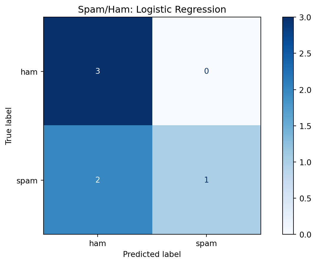
• Example: Trained logistic regression on a toy spam/ham dataset.
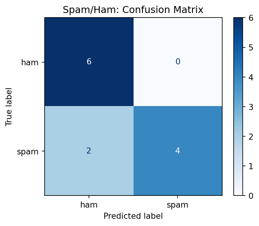
• We evaluate predictions with a confusion matrix before running significance tests.

• Highlight that small differences in results (e.g., 0.5% accuracy gain) may not be meaningful unless tested for significance, due to sampling noise and variance.

Statistical significance testing is essential for validating NLP experiment results. (2/8)

• Statistical hypothesis testing quantifies whether observed performance differences are likely due to chance.
  • Null hypothesis \(H_0\): No difference between systems’ true performance.
  • \(p\)-value: Probability of observing results at least as extreme as those measured, assuming \(H_0\) is true.

• Explain the role of the null hypothesis and \(p\)-values in interpreting whether results are likely due to chance.

Statistical significance testing is essential for validating NLP experiment results. (3/8)

• In NLP, model evaluation metrics (e.g., accuracy, F1) are subject to sampling noise.
  • Random train/test splits and annotation errors introduce variance.
  • Without significance testing, small metric improvements may be spurious.
• Example:
  • Comparing two classifiers with 80.2% vs. 80.7% accuracy on a test set of size \(N\).
  • Is the 0.5% difference meaningful, or within random variation?

• Clarify that methods like bootstrap confidence intervals and paired significance tests help assess the reliability and robustness of findings, especially across multiple datasets.

Statistical significance testing is essential for validating NLP experiment results. (4/8)

Methods like bootstrap confidence intervals and tests across datasets assess result reliability.

• The bootstrap estimates confidence intervals by repeatedly resampling the test set:

\[ \text{For } b = 1, \dots, B: \quad \text{Sample with replacement to create set } D_b \]

\[ \text{Compute metric: } \theta^{(b)} = \text{Metric}(D_b) \]

\[ \text{Form empirical distribution: } \{\theta^{(1)}, \dots, \theta^{(B)}\} \]

• Address the misconception that reporting a higher score alone is sufficient—stress the importance of including test set size, confidence intervals, and statistical test details for proper scientific reporting.

Statistical significance testing is essential for validating NLP experiment results. (6/8)

• Significance testing across datasets (e.g., paired \(t\)-test, approximate randomization) accounts for correlation and variance:
  • Paired \(t\)-test: Compare metric differences per example across systems.
  • Randomization: Shuffle system outputs to simulate null hypothesis.
• Application:
  • Dror et al. (2017) recommend testing across multiple datasets for robustness.

• Transition: Next, we’ll look at best practices for experimental design and reporting standards to further ensure trustworthy results in NLP research.

Statistical significance testing is essential for validating NLP experiment results. (7/8)

Proper significance reporting ensures replicability and trust in classification experiments.

• Reporting standards include:
  • Declaring test set size, number of runs, and test statistic used.
  • Reporting confidence intervals, not just point estimates.

Statistical significance testing is essential for validating NLP experiment results. (8/8)

• Replicability crisis in NLP highlights the necessity of statistical rigor.

• Example reporting statement:

  • “System A outperforms System B on F1 (\(p = 0.03\), 95% CI: [0.02, 0.08]) across 10 datasets.”

Spam/ham: are point estimates enough?

• Confusion matrix + point metrics on the tiny test set.
• Are these point estimates enough to claim a meaningful result?

Metric	Mean
Accuracy	0.838333
Precision	0.996000
Recall	0.678105
F1	0.789740

• Ask students whether these numbers feel reliable given the tiny test set.

Spam/ham: bootstrap confidence intervals

• Now include 95% CIs from bootstrap resampling.
• Given the CIs, how confident are you in the model’s performance?

Metric	Mean	CI Low	CI High
Accuracy	0.838333	0.583333	1.000000
Precision	0.996000	1.000000	1.000000
Recall	0.678105	0.250000	1.000000
F1	0.789740	0.400000	1.000000

• Emphasize that small test sets yield wide confidence intervals.
• Prompt: “Would you change anything about the experiment?”

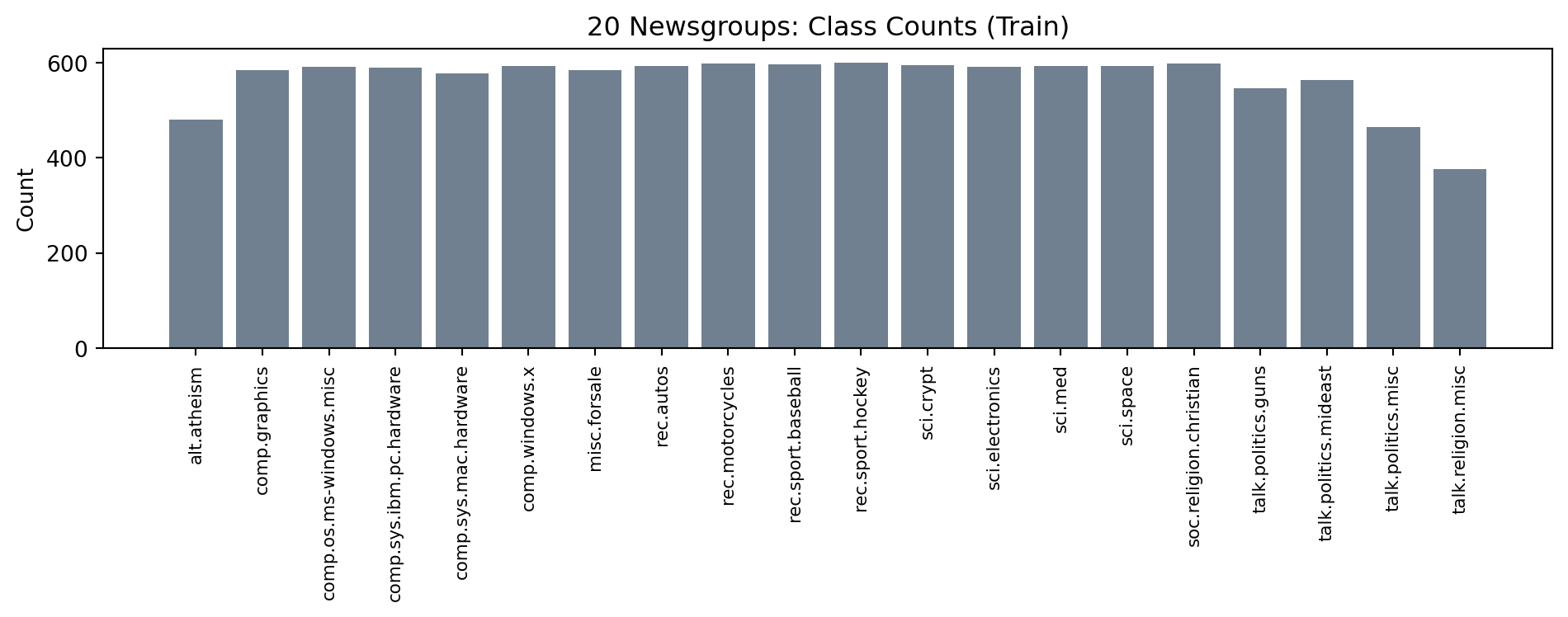
Part 4: Case Study: 20 Newsgroups Classification

20 Newsgroups: classification task

• Predict the discussion group label from the post text.
• Usenet posts from 20 topical forums (sports, politics, tech, religion).
• 20 categories, balanced enough that accuracy is meaningful.
• We strip headers/footers/quotes to focus on content.

Dataset overview

• Train/test splits come from scikit-learn’s fetch_20newsgroups.
• Each example is a short, noisy, user-generated post.

Train size: 11314  Test size: 7532
Classes: 20

Example posts (truncated)

• Look for topical keywords that hint at the group label.

[rec.autos] I was wondering if anyone out there could enlighten me on this car I saw the other day. It was a 2-door sports car, looked to be from the late 60s/ early 70s. It was called a...

[comp.sys.mac.hardware] --

[comp.graphics] Hello, I am looking to add voice input capability to a user interface I am developing on an HP730 (UNIX) workstation. I would greatly appreciate information anyone would care to...

Bigram example: phrase cues

• Bigrams capture short phrases (e.g., “space shuttle”, “power supply”).

Example bigrams: ['60s early' 'info funky' 'know tellme' 'late 60s' 'looked late'
 'looking car' 'model engine' 'production car' 'really small' 'saw day']

Class distribution (train split)

• Classes are roughly balanced, but not perfectly uniform.

Model A: TF-IDF unigrams + L2 logistic regression

• TF-IDF reduces weight on common terms.
• L2 regularization discourages overly large weights.
• Strong baseline with relatively compact feature space.

Model B: TF-IDF unigrams+bigrams + L1 logistic regression

• Bigrams add short-phrase cues.
• L1 encourages sparse, feature-selective weights.
• More features, higher risk of overfitting on small topics.

Accuracy + micro/macro precision/recall/F1

• Micro averages track overall correctness; macro highlights per-class balance.
• Micro: pool all predictions, then compute global \(P/R/F_1\) from total TP/FP/FN.
• Macro: compute \(P/R/F_1\) per class, then average (each class equal weight).

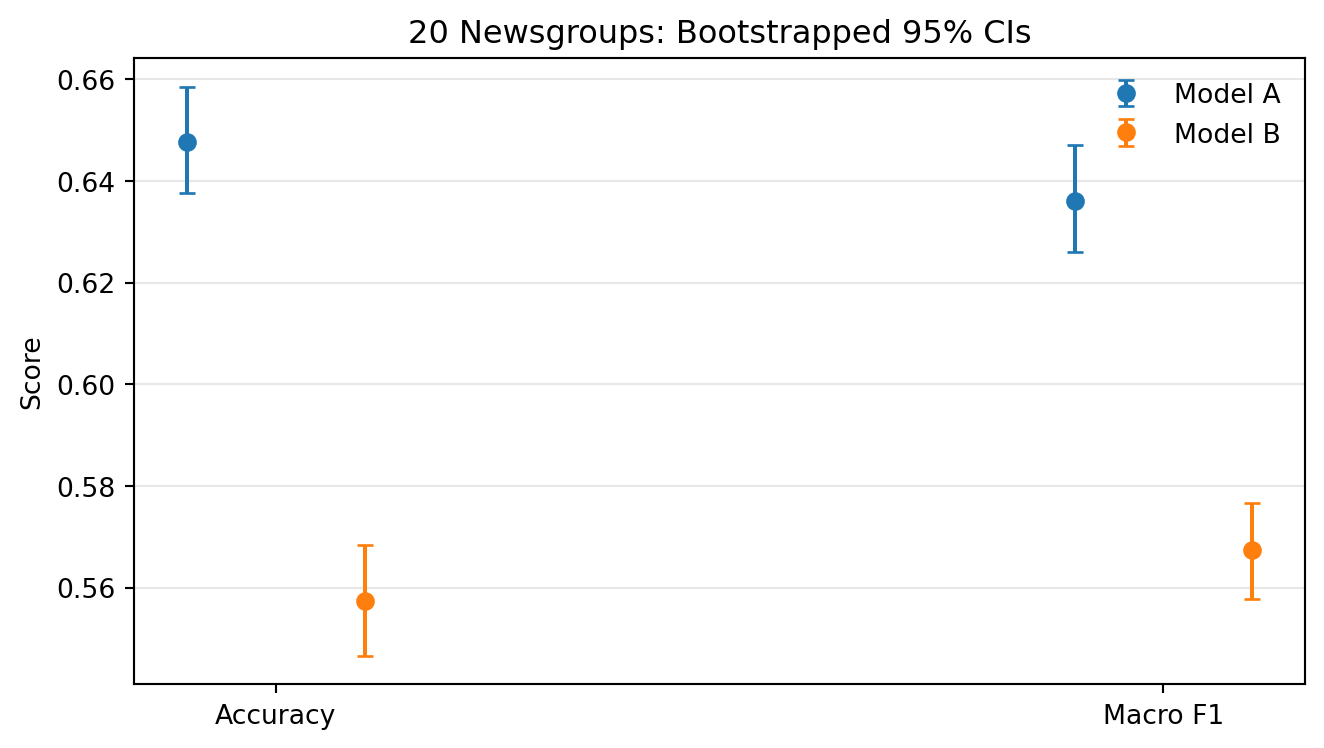
Model A: acc=0.648
  micro: P=0.648 R=0.648 F1=0.648
  macro: P=0.650 R=0.635 F1=0.636
Model B: acc=0.557
  micro: P=0.557 R=0.557 F1=0.557
  macro: P=0.619 R=0.546 F1=0.567

\(F_\beta\) emphasizes recall when \(\beta > 1\)

• Example: \(F_2\) weights recall higher than precision.
• Useful when missing a topic is costlier than a false alarm.

Model A F2: 0.634
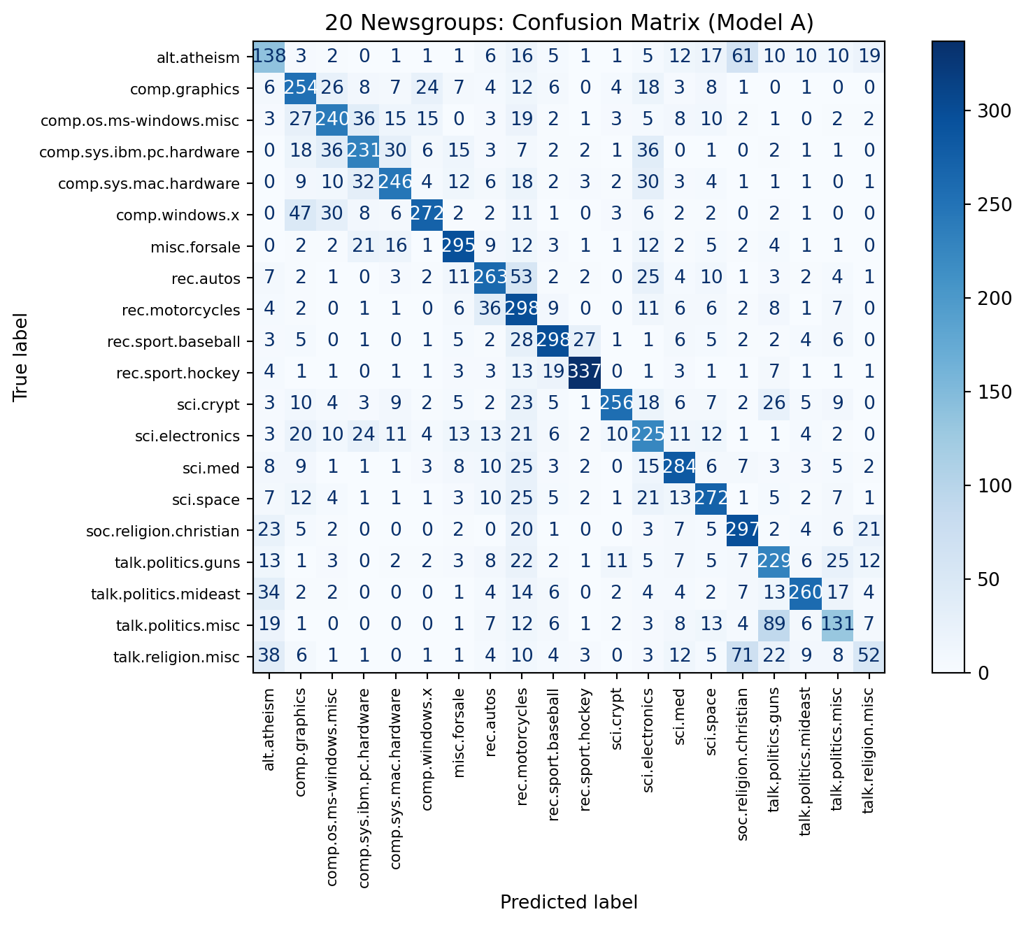
Model B F2: 0.550

Confusion matrix (best macro F1)

Bootstrapped confidence intervals

• 95% CIs for accuracy and macro F1.
• Overlapping intervals would suggest weak evidence of a difference.

Model comparison takeaways

• Model A is a strong, simple baseline with fewer features.
• Model B adds phrase cues but can trade speed for sparsity.
• Macro metrics and the confusion matrix show where each model struggles.

• If you care about interpretability or sparsity, L1 with bigrams is attractive.