Text Classification

Author

Robert Minneker

Published

January 11, 2026

Content derived from: J&M Ch. 4

Note: This is a living draft document

Part 1: Foundations of Text Classification

Definitions and Problem Formulation

Executive Summary

Text classification is the task of assigning predefined labels to text documents, a foundational problem in NLP.
Classification tasks come in several flavors: binary, multiclass, and multilabel, each with distinct mathematical formulations.
Most modern text classification is framed as a supervised learning problem: the goal is to learn a function that maps text inputs to labels, given labeled training data.

What Is Text Classification?

Key Takeaway: Text classification is the process of automatically assigning one or more categories (labels) to a given text input (such as a sentence, paragraph, or document).

Text classification is among the most fundamental problems in natural language processing (NLP). It enables machines to “understand” and organize text by sorting documents, emails, tweets, or any textual data into categories. These categories might be as broad as “spam” vs. “not spam,” as nuanced as “positive,” “negative,” or “neutral” sentiment, or as complex as a set of topics relevant to the document.

Motivation: Why Do We Need Text Classification?

Key Takeaway: Text classification automates decisions that would otherwise require manual reading and sorting, enabling large-scale analysis of text data.

Common Use Cases

Spam Detection: Automatically identifying and filtering unwanted emails.
Sentiment Analysis: Determining the emotional tone of product reviews, social media posts, etc.
Topic Labeling: Tagging news articles or scientific papers with subject areas.
Toxicity Detection: Filtering out offensive or inappropriate comments.
Intent Detection: Understanding user queries in chatbots or virtual assistants.

Note: Text classification systems have real-world consequences: their mistakes (e.g., misclassifying hate speech as benign) can impact user experience, safety, or fairness.

Types of Text Classification Tasks

Key Takeaway: Classification tasks are not all the same. Understanding the distinctions between binary, multiclass, and multilabel classification is crucial for selecting the right model and loss function.

1. Binary Classification

Definition: Each input is assigned to one of two possible classes.
Examples:
Is this email spam (spam vs. not spam)?
Is this product review positive (positive vs. not positive)?

2. Multiclass Classification

Definition: Each input is assigned to one and only one of three or more classes.
Examples:
What is the topic of this news article? (sports, politics, technology, etc.)
Which language is this sentence written in? (English, French, German, …)

3. Multilabel Classification

Definition: Each input can be assigned multiple labels simultaneously.
Examples:
What topics does this research paper cover? (machine learning, linguistics, ethics)
What emotions are present in this tweet? (joy, anger, surprise)

Important: Multilabel tasks require special handling: the output is a vector of independent binary decisions (one per label), not a single categorical choice.

Formal Problem Formulation

Key Takeaway: Text classification is typically formulated as a supervised learning problem: given a dataset of \((x, y)\) pairs, learn a function \(f\) that maps input texts \(x\) to labels \(y\).

Inputs and Outputs

Input: A text document, sentence, or utterance, denoted as \(x\).
Output: A label \(y\) (or a set of labels), indicating the class(es) to which \(x\) belongs.

Feature Representation

Before a machine can classify text, it must convert the input \(x\) into a feature vector:

Denote the feature vector as \(\vec{x} = [x_1, x_2, ..., x_n]\).
Features can be simple (e.g., word counts, n-grams) or complex (e.g., embeddings from a neural network).

The Classifier Function

The model learns a function \(f\):

\[ f: \vec{x} \mapsto y \]

For binary/multiclass: \(y\) is a single label.
For multilabel: \(y\) is a set or vector of labels.

Training Objective

The model’s parameters (e.g., weights \(\vec{w}\), bias \(b\)) are learned by minimizing a loss function over the training data. For probabilistic classifiers:

Binary: Use sigmoid (\(\sigma\)) to produce \(P(y=1 \mid \vec{x})\).
Multiclass: Use softmax to produce \(P(y=k \mid \vec{x})\) for \(k\) classes.

Let \(\mathcal{D} = \{(\vec{x}^{(i)}, y^{(i)})\}_{i=1}^N\) be the training set.

Goal: Find parameters \(\theta\) (e.g., \(\vec{w}\) and \(b\)) that minimize the expected loss:

\[ \theta^* = \arg\min_{\theta} \frac{1}{N} \sum_{i=1}^N \mathcal{L}(f_\theta(\vec{x}^{(i)}), y^{(i)}) \]

Where \(\mathcal{L}\) is a suitable loss function (e.g., cross-entropy).

import torch
import torch.nn as nn

# Toy corpus and binary labels
texts = ["free money", "hi friend", "limited offer"]
labels = torch.tensor([1, 0, 1], dtype=torch.float32)

# Build a tiny bag-of-words vocab
vocab = {w: i for i, w in enumerate(sorted(set(" ".join(texts).split())))}

def vectorize(text):
    vec = torch.zeros(len(vocab))
    for w in text.split():
        vec[vocab[w]] += 1.0
    return vec

X = torch.stack([vectorize(t) for t in texts])  # (n_samples, n_features)

# Linear classifier = logistic regression in PyTorch
model = nn.Linear(X.shape[1], 1)
loss_fn = nn.BCEWithLogitsLoss()  # sigmoid + cross-entropy
optimizer = torch.optim.SGD(model.parameters(), lr=0.1)

logits = model(X).squeeze(1)
loss = loss_fn(logits, labels)
loss.backward()
optimizer.step()

Placeholder for a simple PyTorch text classification model, showing input preprocessing, model definition, and training loop.
Each code line should be annotated in prose to explain the logic, especially the parts mapping input text to features and labels.

Check Your Understanding

Classification Task Types: Why would you choose a multilabel classification approach over multiclass for a news categorization task? What are the practical consequences for model design and evaluation?
Feature Representation: How does the choice of feature representation (e.g., bag-of-words vs. contextual embeddings) affect the ability of a classifier to distinguish between subtle categories, such as sarcasm detection?
Loss Functions and Outputs: Suppose you are building a classifier for toxic comment detection that allows comments to be both toxic and obscene. What loss function and output activation should you use, and why?

import numpy as np
from sklearn.feature_extraction.text import CountVectorizer
from sklearn.linear_model import LogisticRegression

def spam_classifier(docs, labels, new_doc):
    """
    Trains a binary text classifier and predicts label for a new document.
    Args:
      docs: list of training documents (strings)
      labels: list of binary labels (0 or 1)
      new_doc: a single document to classify
    Returns:
      predicted label (0 or 1) for new_doc
    """
    vectorizer = CountVectorizer()  # Convert text to bag-of-words features
    X = vectorizer.fit_transform(docs)
    clf = LogisticRegression()
    clf.fit(X, labels)
    X_new = vectorizer.transform([new_doc])
    return clf.predict(X_new)[0]

# Example usage:
spam_classifier(["free money", "hi friend"], [1, 0], "free offer")

np.int64(1)

import torch
import torch.nn as nn

class MultiLabelModel(nn.Module):
    """
    Simple multilabel classifier with two output labels.
    """
    def __init__(self, input_dim):
        super().__init__()
        self.linear = nn.Linear(input_dim, 2)  # 2 independent outputs

    def forward(self, x):
        return torch.sigmoid(self.linear(x))  # Sigmoid for multilabel

# Example usage:
model = MultiLabelModel(input_dim=4)
input_features = torch.tensor([[0.1, 0.2, 0.3, 0.4]])
output_probs = model(input_features)  # Predicted probabilities for 2 labels

Feature Representation in Text

Executive Summary

Feature representation is the foundation of text classification: Effective models rely on transforming raw text into structured, informative numerical vectors.
Bag-of-Words (BoW), term weighting, and dimensionality reduction are essential: These techniques convert text into vectors, capture word importance, and manage the high dimensionality of language data.
Careful feature selection can make or break your classifier: Choosing the right representation and reducing noise improves both accuracy and efficiency.

Why: The Motivation Behind Feature Representation in Text

Key Takeaway: Transforming text into features is the first and most crucial step for any statistical or neural text classifier. The way we represent text directly determines what patterns a model can learn.

Natural language, in its raw form, is ambiguous, variable, and high-dimensional. Computers require fixed-size, numerical input, but text is a sequence of variable-length symbols. Feature representation bridges this gap: it encodes the essential aspects of text into vectors that can be processed by machine learning algorithms.

The earliest and still widely used strategy is the Bag-of-Words (BoW) model, where each document is represented by the words it contains, disregarding word order. While simple, BoW underpins many effective models and introduces core concepts like term frequency and feature selection.

Applications of text feature representation include:

Spam detection (Is this email spam or not?)
Sentiment analysis (Is this review positive or negative?)
Topic classification (What category does this article belong to?)

How: Mathematical Foundations of Feature Representation

Bag-of-Words and Vector Space Models

Key Takeaway: The Bag-of-Words model represents each document as a vector over the vocabulary, enabling mathematical operations and machine learning.

Let \(V = \{w_1, w_2, ..., w_{|V|}\}\) be the set of all unique words (the vocabulary) in your corpus. Each document \(d\) is represented as a vector \(\mathbf{x} \in \mathbb{R}^{|V|}\), where each entry \(x_j\) quantifies the presence or importance of word \(w_j\) in \(d\).

Basic Bag-of-Words

Multinomial (count) representation:

\[ x_j = \text{count}(w_j, d) \]

Here, \(x_j\) is the number of times word \(w_j\) appears in document \(d\).

Binarized (set-of-words) representation:

\[ x_j = \begin{cases} 1 & \text{if } w_j \in d \\ 0 & \text{otherwise} \end{cases} \]

Note: The BoW model ignores word order, so “dog bites man” and “man bites dog” are represented identically. This is both a limitation and a source of robustness.

Term Frequency and Document Frequency Weighting

Key Takeaway: Not all words are equally informative; weighting schemes like TF-IDF adjust for this.

Term Frequency (TF)

The term frequency of word \(w_j\) in document \(d\) is:

\[ \text{tf}(w_j, d) = \frac{\text{count}(w_j, d)}{\sum_{k=1}^{|V|} \text{count}(w_k, d)} \]

This normalizes for document length.

Inverse Document Frequency (IDF)

The inverse document frequency of word \(w_j\) across a corpus \(D\) is:

\[ \text{idf}(w_j, D) = \log \frac{N}{|\{ d \in D : w_j \in d \}|} \]

where \(N\) is the total number of documents.

TF-IDF Weighting

Combine the above to score word importance:

\[ \text{tfidf}(w_j, d, D) = \text{tf}(w_j, d) \cdot \text{idf}(w_j, D) \]

Tip: Words like “the” or “and” have high term frequency but low informativeness, so their IDF is low, reducing their impact in the final vector.

Binarized vs. Multinomial Representations

Key Takeaway: Choosing between binarized and count-based features depends on the task and model.

Binarized representation captures presence/absence and is robust to word repetition (useful in some classification tasks).
Multinomial representation captures frequency information, which can be informative in longer texts or when word repetition is meaningful.

Important: Naive Bayes classifiers often assume a multinomial model (word counts), but for some tasks, binarized features can outperform, especially when repeated words add little extra information.

Feature Selection and Dimensionality Reduction

Key Takeaway: Feature spaces in text are huge. Selecting the right subset of features improves performance and reduces overfitting.

Why Reduce Dimensionality?

Vocabulary sizes often reach tens of thousands.
Most words are rare or irrelevant for a given task.
High-dimensional vectors can cause computational and statistical issues (“curse of dimensionality”).

Feature Selection Methods

Frequency thresholding: Remove words that are too rare or too common.
Statistical measures: Use \(\chi^2\), mutual information, or information gain to select the most discriminative words.

Dimensionality Reduction Techniques

Principal Component Analysis (PCA): Projects data to lower dimensions, capturing variance.
Latent Semantic Analysis (LSA): Uses Singular Value Decomposition (SVD) on the term-document matrix to uncover latent topics.

Warning: Aggressive feature reduction can remove rare but highly predictive words. Always validate your choices empirically!

Implementation: From Theory to Code

Key Takeaway: Most modern libraries (e.g., scikit-learn, PyTorch) provide utilities for vectorizing text, but understanding the underlying math helps you debug and improve your models.

Placeholder for code showing how to construct BoW and TF-IDF features using standard Python/NLP libraries.
Line-by-line prose will clarify tokenization, vocabulary building, vectorization, and matrix construction.

Synthesis: Check Your Understanding

What are the trade-offs between using a binarized vs. a multinomial Bag-of-Words representation for a sentiment analysis task?
How does the choice of feature selection threshold (e.g., minimum document frequency) impact both model performance and generalization?
Why might dimensionality reduction techniques like LSA sometimes hurt performance on text classification tasks, despite reducing feature space size?

Self-study reflection: Try constructing a Bag-of-Words vector by hand for a short paragraph. Apply both binarized and TF-IDF weighting. How does the feature vector change? What information is gained or lost?

from sklearn.feature_extraction.text import CountVectorizer

def bow_vectorization(docs, binary=False):
    """
    Create Bag-of-Words vectors (count or binary) for a list of documents.
    :param docs: List of text documents.
    :param binary: If True, use binary (presence/absence) features.
    :return: Vocabulary and document-term matrix.
    """
    vectorizer = CountVectorizer(binary=binary)
    dt_matrix = vectorizer.fit_transform(docs)
    vocab = vectorizer.get_feature_names_out()
    return vocab, dt_matrix.toarray()

docs = ["dog bites man", "man bites dog", "dog eats meat"]
vocab, bow_matrix = bow_vectorization(docs, binary=True)
print(vocab)
print(bow_matrix)

['bites' 'dog' 'eats' 'man' 'meat']
[[1 1 0 1 0]
 [1 1 0 1 0]
 [0 1 1 0 1]]

from sklearn.feature_extraction.text import TfidfVectorizer

def tfidf_vectorization(docs):
    """
    Create TF-IDF weighted vectors for a list of documents.
    :param docs: List of text documents.
    :return: Vocabulary and TF-IDF matrix.
    """
    vectorizer = TfidfVectorizer()
    tfidf_matrix = vectorizer.fit_transform(docs)
    vocab = vectorizer.get_feature_names_out()
    return vocab, tfidf_matrix.toarray()

docs = ["dog bites man", "man bites dog", "dog eats meat"]
vocab, tfidf_matrix = tfidf_vectorization(docs)
print(vocab)
print(tfidf_matrix)

['bites' 'dog' 'eats' 'man' 'meat']
[[0.61980538 0.48133417 0.         0.61980538 0.        ]
 [0.61980538 0.48133417 0.         0.61980538 0.        ]
 [0.         0.38537163 0.65249088 0.         0.65249088]]

Evaluation Metrics

TL;DR

Evaluation metrics provide quantitative ways to assess the performance of text classifiers, guiding model selection and improvement.
Accuracy, precision, recall, and F-measure offer complementary perspectives, especially important when dealing with imbalanced data.
Confusion matrices and cross-validation are essential tools for interpreting results and ensuring reliable, generalizable findings.

Why Do We Need Evaluation Metrics?

Key Takeaway: Evaluation metrics are not just numbers—they shape what we optimize, how we compare models, and which real-world mistakes we prioritize.

Imagine building a spam filter. If it labels every email as “not spam,” it might still be “accurate” if most emails aren’t spam—but it’s also useless. This exposes a core issue in text classification: not all errors are equal.

Some mistakes (missing a cancer diagnosis, failing to flag hate speech) are much costlier than others.
Simple accuracy can mislead us, especially when the data is imbalanced or when the stakes differ for different types of errors.

Evaluation metrics let us:

Decide which model is “best” for our goals.
Understand the strengths and weaknesses of a model.
Tune and improve models in a principled way.

The How: Metrics, Math, and Interpretation

The Confusion Matrix

Key Takeaway: The confusion matrix is the starting point for nearly all evaluation metrics. It organizes predictions into four categories, making error analysis concrete.

For binary classification (e.g., spam/not spam), the confusion matrix is:

\[ \begin{array}{c|cc} \text{Actual}~\vert~\text{Predicted} & \text{Positive} & \text{Negative} \\ \hline \text{Positive} & \text{TP} & \text{FN} \\ \text{Negative} & \text{FP} & \text{TN} \\ \end{array} \]

Where:

\(\text{TP}\): True Positives (correctly predicted positive)
\(\text{FP}\): False Positives (incorrectly predicted positive)
\(\text{FN}\): False Negatives (missed positive)
\(\text{TN}\): True Negatives (correctly predicted negative)

Accuracy

Key Takeaway: Accuracy is the most intuitive metric but can be misleading for skewed datasets.

Defined as the proportion of correct predictions:

\[ \text{Accuracy} = \frac{\text{TP} + \text{TN}}{\text{TP} + \text{TN} + \text{FP} + \text{FN}} \]

Pitfall: If only 1% of emails are spam, a model that always predicts “not spam” achieves 99% accuracy—but never catches spam.

Precision and Recall

Key Takeaway: Precision and recall help us analyze specific types of errors, especially in imbalanced or high-stakes settings.

Precision: Of all items predicted positive, how many were actually positive?

\[ \text{Precision} = \frac{\text{TP}}{\text{TP} + \text{FP}} \]

High precision: few false alarms.

Recall: Of all actual positives, how many did we catch?

\[ \text{Recall} = \frac{\text{TP}}{\text{TP} + \text{FN}} \]

High recall: few misses.

Example: In medical diagnosis, recall (sensitivity) is crucial—you don’t want to miss actual cases. In spam filtering, you may prioritize precision to avoid flagging important emails.

F-measure (\(F_\beta\) and \(F_1\) Score)

Key Takeaway: The F-measure combines precision and recall into a single, tunable score.

The general \(F_\beta\) score is:

\[ F_\beta = (1 + \beta^2) \cdot \frac{\text{Precision} \cdot \text{Recall}}{(\beta^2 \cdot \text{Precision}) + \text{Recall}} \]

\(\beta\) controls the trade-off: \(\beta > 1\) weights recall higher, \(\beta < 1\) weights precision higher.
The most common case is \(\beta = 1\) (the \(F_1\) score):

\[ F_1 = 2 \cdot \frac{\text{Precision} \cdot \text{Recall}}{\text{Precision} + \text{Recall}} \]

Tip: Use \(F_1\) when you want a single metric that balances precision and recall. Adjust \(\beta\) if one is more important for your application.

Considerations for Imbalanced Data

Key Takeaway: When classes are imbalanced, accuracy is often uninformative. Focus on precision, recall, and F-measure.

Suppose only 1% of news articles are about disasters. A classifier that always predicts “not disaster” is 99% accurate, but useless. In such cases:

Evaluate using \(F_1\) or area under the precision-recall curve.
Consider class-specific metrics (e.g., recall for the minority class).

Warning: Always inspect the confusion matrix for imbalanced data. A high accuracy may hide systematic failures on rare but critical classes.

Cross-Validation Strategies

Key Takeaway: Cross-validation gives robust estimates of performance and helps avoid overfitting.

\(k\)-fold cross-validation:

Split data into \(k\) equal parts (“folds”).
Train on \(k-1\) folds, evaluate on the held-out fold.
Repeat \(k\) times, each time with a different held-out fold.
Report the average metric (e.g., average \(F_1\)).

\[ \text{Mean } F_1 = \frac{1}{k} \sum_{i=1}^k F_1^{(i)} \]

Stratified \(k\)-fold cross-validation: Ensures each fold has a similar class distribution as the full dataset—especially important for imbalanced data.

Important: Always use cross-validation on training data only. Test data should be held out until final evaluation, to avoid “leakage.”

Synthesis: Check Your Understanding

Why might accuracy be misleading for rare-event classification tasks? Discuss with reference to the confusion matrix and real-world consequences.
Suppose your classifier has high precision but low recall on a medical diagnosis task. What are the practical implications? How might you address this?
Describe the difference between standard \(k\)-fold and stratified \(k\)-fold cross-validation. In what scenarios is stratification critical?

import numpy as np

def basic_metrics(y_true, y_pred):
    """
    Computes confusion matrix, precision, recall, and F1 for binary labels.
    """
    tp = np.sum((y_true == 1) & (y_pred == 1))  # True Positives
    fp = np.sum((y_true == 0) & (y_pred == 1))  # False Positives
    fn = np.sum((y_true == 1) & (y_pred == 0))  # False Negatives

    precision = tp / (tp + fp) if (tp + fp) > 0 else 0.0
    recall = tp / (tp + fn) if (tp + fn) > 0 else 0.0
    f1 = 2 * precision * recall / (precision + recall) if (precision + recall) > 0 else 0.0
    return precision, recall, f1

# Example usage
y_true = np.array([1, 0, 1, 1, 0, 0, 1])
y_pred = np.array([1, 0, 1, 0, 0, 1, 0])
print(basic_metrics(y_true, y_pred))

(np.float64(0.6666666666666666), np.float64(0.5), np.float64(0.5714285714285715))

from sklearn.model_selection import StratifiedKFold

def stratified_split(labels, k=3):
    """
    Yields stratified train/test indices for each fold.
    """
    skf = StratifiedKFold(n_splits=k, shuffle=True, random_state=42)
    for train_idx, test_idx in skf.split(range(len(labels)), labels):
        yield train_idx, test_idx

# Example usage
labels = [0, 0, 0, 1, 0, 1, 0, 0, 1]
for train_idx, test_idx in stratified_split(labels, k=3):
    print("Train:", train_idx, "Test:", test_idx)

Train: [2 3 4 5 6 7] Test: [0 1 8]
Train: [0 1 2 5 6 8] Test: [3 4 7]
Train: [0 1 3 4 7 8] Test: [2 5 6]

Part 2: Logistic Regression

Discriminative Models

TL;DR

Discriminative models directly model the probability of a label given the input (\(P(y|x)\)), as opposed to modeling the input itself.
Logistic regression is a canonical discriminative model for binary text classification, relying on feature engineering.
Choosing discriminative vs. generative approaches impacts the type of information the model learns and how it handles ambiguity in natural language.

Key Takeaway

Discriminative models focus on learning the boundary between classes, not the process that generates the data itself. Logistic regression exemplifies this by directly estimating \(P(y \mid x)\) using features extracted from the input, making it a natural fit for many NLP classification tasks.

Why: Motivation for Discriminative Models in NLP

Natural language is ambiguous and highly variable. In text classification tasks—such as spam detection, sentiment analysis, or topic categorization—the goal is to assign the most probable label to a given document or sentence. Here, what matters most is the relationship between features in the text (e.g., presence of specific words or patterns) and the correct label.

Discriminative vs. Generative: The Core Distinction

Generative models (like Naive Bayes) model the joint probability \(P(x, y)\) or, equivalently, \(P(x \mid y)P(y)\). They try to capture how the data is generated for each class.
Discriminative models (like logistic regression) directly model the conditional probability \(P(y \mid x)\), focusing on the boundary between classes.

Note: In many NLP tasks, the data distribution \(P(x)\) is complex and high-dimensional, making it hard to model directly. Discriminative models sidestep this by focusing only on what matters for classification: \(P(y \mid x)\).

Intuitive Example

Suppose you’re building a spam filter. A discriminative model asks: Given these words in an email, how likely is it to be spam? It doesn’t try to model how legitimate or spam emails are composed in general, just the boundary between the two.

How: Mathematical Formulation of Discriminative Models

Formal Definition

A discriminative model seeks to estimate \(P(y \mid x)\), where:

\(x\) is an input feature vector (e.g., representation of a document)
\(y\) is a label (e.g., spam or not spam)

Logistic Regression as a Discriminative Model

For binary classification (\(y \in \{0, 1\}\)), logistic regression defines:

\[ P(y = 1 \mid x) = \sigma(w \cdot x + b) = \frac{1}{1 + e^{-(w \cdot x + b)}} \]

where:

\(x = [x_1, x_2, ..., x_n]\) is the feature vector for an input (e.g., word counts, n-grams)
\(w = [w_1, w_2, ..., w_n]\) are the learned weights
\(b\) is a bias term
\(\sigma\) is the sigmoid function

The classifier assigns label \(1\) if \(P(y=1 \mid x) > 0.5\), and \(0\) otherwise.

Objective Function

To train the model, we minimize the cross-entropy loss (also called log loss):

\[ L(w, b) = -\sum_{i=1}^m \left[ y^{(i)} \log \hat{y}^{(i)} + (1 - y^{(i)}) \log (1 - \hat{y}^{(i)}) \right] \]

where \(\hat{y}^{(i)} = \sigma(w \cdot x^{(i)} + b)\).

Feature Engineering

Features are crucial in discriminative models. Examples include:

Bag-of-words: \(x_j\) is the count or presence of word \(j\).
N-gram features: \(x_j\) counts occurrences of a particular phrase.
Domain-specific patterns: e.g., presence of URLs, exclamation marks for spam detection.

Tip: The quality and choice of features often have more impact on performance than the choice of discriminative model itself, especially for logistic regression.

Implementation: Logistic Regression in Practice

Pipeline Steps

Feature Extraction: Convert raw text into a feature vector \(x\) for each example.
Model Training: Optimize weights \(w\) and bias \(b\) using stochastic gradient descent to minimize cross-entropy loss.
Prediction: For a new input \(x\), compute \(\hat{y} = \sigma(w \cdot x + b)\).

Important: In modern NLP, feature extraction may use more complex embeddings (e.g., from Transformers), but the discriminative paradigm—directly modeling \(P(y \mid x)\)—remains foundational.

Synthesis: Check Your Understanding

Boundary Learning: Why might a discriminative model outperform a generative model on text classification tasks with highly overlapping class distributions?
Feature Impact: Suppose you add a new feature to your model (e.g., a word indicating strong sentiment). How does logistic regression incorporate and assign weight to this new feature during training?
Limitation Scenario: Can you think of an NLP task where modeling \(P(x \mid y)\) (generative) might be preferable to \(P(y \mid x)\) (discriminative)? Why?

import numpy as np
from sklearn.linear_model import LogisticRegression

def simple_logistic_regression():
    """
    Minimal example: Discriminative text classification with logistic regression.
    Classifies short texts as spam/not-spam based on presence of 'offer'.
    """
    # Feature: [contains 'offer']
    X = np.array([[1], [0], [1], [0]])  # 1 if 'offer' present, else 0
    y = np.array([1, 0, 1, 0])          # 1 = spam, 0 = not spam

    model = LogisticRegression()
    model.fit(X, y)
    # Predict if 'offer' present in new email
    pred = model.predict([[1]])
    print("Spam prediction for 'offer':", pred[0])

import numpy as np

def manual_sigmoid_logistic_regression():
    """
    Manually computes P(y=1|x) for a single feature using logistic regression.
    Shows discriminative modeling of P(y|x).
    """
    def sigmoid(z):
        return 1 / (1 + np.exp(-z))

    # Suppose feature x=2 (e.g., word count), w=1.5, b=-2
    x = 2
    w = 1.5
    b = -2
    score = w * x + b
    prob = sigmoid(score)
    print("Probability y=1 given x=2:", prob)

Binary Logisitic Regression

Executive Summary

Logistic regression is the canonical model for binary classification tasks, mapping feature vectors to probabilities via the sigmoid function.
The model parameters are estimated by maximizing the likelihood (minimizing cross-entropy loss), typically via gradient descent methods.
Regularization (L1, L2) is crucial to prevent overfitting and encourage model generalization.

The “Why”: Motivation for Binary Logistic Regression

Key Takeaway: Logistic regression solves the problem of predicting a binary label (e.g., spam or not, positive or negative sentiment) from a set of input features, providing not just a decision but a calibrated probability.

Binary classification is foundational in NLP and machine learning. Tasks like spam detection, sentiment analysis, and topic classification all boil down to predicting whether an input belongs to class \(1\) (positive) or class \(0\) (negative). Unlike linear regression, which predicts real values, we want our outputs to represent probabilities and be constrained between \(0\) and \(1\).

Why not just threshold the output of a linear model? Because linear models can produce any real number, leading to nonsensical probabilities (e.g., \(-1.2\) or \(3.7\)). We need a function that smoothly maps any real-valued input to the \((0,1)\) interval. Enter the sigmoid.

The “How” (Math): Model, Loss, and Optimization

Key Takeaway: Logistic regression models \(P(y=1|x)\) using a sigmoid-transformed linear function. Parameter learning is framed as maximizing the likelihood (or minimizing the cross-entropy loss), typically with gradient descent.

Model Formulation

Given a feature vector \(x \in \mathbb{R}^n\) and label \(y \in \{0,1\}\), the logistic regression model defines:

\[ z = w \cdot x + b \]

\[ \hat{y} = \sigma(z) = \frac{1}{1 + e^{-z}} \]

where:

\(w\) is the weight vector,
\(b\) is the bias (intercept),
\(\sigma(\cdot)\) is the sigmoid function.

The output \(\hat{y}\) is interpreted as the estimated probability that \(y=1\) given \(x\).

Likelihood Function

Assuming independent training examples \(\{(x^{(i)}, y^{(i)})\}_{i=1}^m\), the likelihood of the observed labels is:

\[ L(w, b) = \prod_{i=1}^m P(y^{(i)}|x^{(i)}; w, b) \]

For each example, the conditional probability is:

\[ P(y|x) = \hat{y}^y (1 - \hat{y})^{1-y} \]

Log-Likelihood and Cross-Entropy Loss

Working with logs for numerical stability, we maximize the log-likelihood:

\[ \ell(w, b) = \sum_{i=1}^m \left[ y^{(i)} \log \hat{y}^{(i)} + (1 - y^{(i)}) \log (1 - \hat{y}^{(i)}) \right] \]

Equivalently, we minimize the cross-entropy loss:

\[ J(w, b) = -\frac{1}{m} \sum_{i=1}^m \left[ y^{(i)} \log \hat{y}^{(i)} + (1 - y^{(i)}) \log (1 - \hat{y}^{(i)}) \right] \]

This loss penalizes confident but incorrect predictions much more heavily than less confident ones.

Parameter Estimation: Gradient Descent

We seek \(w, b\) that minimize \(J(w, b)\). The gradients are:

\[ \frac{\partial J}{\partial w_j} = \frac{1}{m} \sum_{i=1}^m \left( \hat{y}^{(i)} - y^{(i)} \right) x_j^{(i)} \]

\[ \frac{\partial J}{\partial b} = \frac{1}{m} \sum_{i=1}^m \left( \hat{y}^{(i)} - y^{(i)} \right) \]

These gradients drive the update steps in (stochastic) gradient descent.

Regularization (L1 and L2)

To improve generalization and prevent overfitting, we often add a regularization term to the loss:

L2 regularization (Ridge):

\[ J_{L2}(w, b) = J(w, b) + \lambda \|w\|_2^2 \]

L1 regularization (Lasso):

\[ J_{L1}(w, b) = J(w, b) + \lambda \|w\|_1 \]

\(\lambda\) controls the strength of regularization.

Tip: L1 regularization promotes sparsity (feature selection), while L2 shrinks weights but usually keeps all features in play.

The “Implementation” (Code)

Key Takeaway: Modern frameworks like PyTorch make it straightforward to implement logistic regression, but understanding the math is crucial for debugging and customizing.

import torch
import torch.nn as nn

# Binary logistic regression with L2 regularization (weight_decay)
X = torch.randn(8, 4)
y = torch.tensor([0, 1, 0, 1, 0, 1, 0, 1], dtype=torch.float32)

model = nn.Linear(4, 1)
loss_fn = nn.BCEWithLogitsLoss()
optimizer = torch.optim.SGD(model.parameters(), lr=0.1, weight_decay=1e-3)

optimizer.zero_grad()
logits = model(X).squeeze(1)
loss = loss_fn(logits, y)
loss.backward()
optimizer.step()

The core implementation involves defining a linear layer, applying the sigmoid, and using binary cross-entropy loss.
Optimizers (e.g., SGD, Adam) handle parameter updates.
For regularization, add the appropriate penalty to the loss before calling .backward().

The “Synthesis”: Check Your Understanding

Why is the sigmoid function specifically chosen for binary logistic regression, and what would go wrong if we used a different function (e.g., \(\tanh\) or ReLU)?
Derive the gradient of the cross-entropy loss with respect to the weights \(w\) from first principles. Why does this gradient have a particularly simple form?
Compare and contrast the effects of L1 and L2 regularization in the context of text classification with high-dimensional sparse features (e.g., bag-of-words). When might you prefer one over the other?

Common Pitfall: Failing to shuffle your data or using inappropriate learning rates can cause SGD to converge slowly or get stuck in poor local minima. Always monitor your loss curves and validate on held-out data.

import numpy as np

def logistic_regression_step(X, y, w, b, lr=0.1):
    """
    Perform one gradient descent step for binary logistic regression.
    X: features (n_samples x n_features)
    y: labels (n_samples,)
    w: weights (n_features,)
    b: bias (scalar)
    lr: learning rate
    Returns updated w, b.
    """
    z = X @ w + b                      # Linear combination
    y_pred = 1 / (1 + np.exp(-z))      # Sigmoid activation
    error = y_pred - y                 # Prediction error
    w -= lr * (X.T @ error) / len(y)   # Gradient update for weights
    b -= lr * np.mean(error)           # Gradient update for bias
    return w, b

import torch
import torch.nn as nn

class MiniLogReg(nn.Module):
    """
    Minimal binary logistic regression using PyTorch.
    """
    def __init__(self, n_features):
        super().__init__()
        self.linear = nn.Linear(n_features, 1)
    
    def forward(self, x):
        return torch.sigmoid(self.linear(x))  # Sigmoid maps output to (0, 1)

Multiclass Logistic Regression

Executive Summary

Multiclass logistic regression extends binary logistic regression to classification tasks with more than two classes, using strategies like one-vs-rest and softmax regression.
The softmax function generalizes the sigmoid, converting raw model outputs into a probability distribution over all possible classes.
Training involves minimizing the cross-entropy loss using algorithms like stochastic gradient descent, with practical considerations for class imbalance and implementation efficiency.

The “Why”: Motivation for Multiclass Logistic Regression

Key Takeaway: Many real-world NLP problems require choosing among more than two categories—think topic classification, intent detection, or part-of-speech tagging. Multiclass logistic regression provides a probabilistic, interpretable, and scalable approach for these tasks.

Why Not Just Use Binary Logistic Regression?

Binary logistic regression predicts the probability that an input \(x\) belongs to class \(1\) versus class \(0\). But what if you have three, four, or even a hundred classes?

Example: In topic classification, you might have documents labeled as sports, politics, science, and entertainment.
Limitation: Binary logistic regression can’t natively handle more than two classes.

Approaches to Multiclass Classification

There are two primary strategies:

One-vs-Rest (OvR): Train a separate binary classifier for each class. For class \(k\), the classifier predicts whether an example is in class \(k\) or not. At prediction time, pick the class with the highest score.
Softmax Regression (a.k.a. Multinomial Logistic Regression): Train a single model that simultaneously considers all classes, using the softmax function to output a probability distribution over classes.

The “How”: Mathematical Foundations

Key Takeaway: Softmax regression models the probability of each class as a normalized exponential of linear functions of the input, enabling direct multiclass probability modeling.

Model Definition

Suppose we have \(K\) possible classes, labeled \(1, 2, ..., K\). For an input feature vector \(\mathbf{x} \in \mathbb{R}^d\), the model computes a score for each class:

\[ z_k = \mathbf{w}_k^\top \mathbf{x} + b_k \qquad \text{for } k = 1, \ldots, K \]

where \(\mathbf{w}_k\) and \(b_k\) are the weights and bias for class \(k\).

Softmax Function

The softmax function converts these scores into a probability distribution:

\[ P(y = k \mid \mathbf{x}) = \frac{\exp(z_k)}{\sum_{j=1}^K \exp(z_j)} \]

Each \(P(y = k \mid \mathbf{x})\) is in \([0,1]\) and \(\sum_{k=1}^K P(y = k \mid \mathbf{x}) = 1\).

Cross-Entropy Loss

Given a one-hot encoded true label vector \(\mathbf{y}\) for input \(\mathbf{x}\), the cross-entropy loss for a single training example is:

\[ \mathcal{L}(\mathbf{y}, \hat{\mathbf{y}}) = -\sum_{k=1}^K y_k \log \hat{y}_k \]

Here, \(\hat{y}_k = P(y = k \mid \mathbf{x})\), and \(y_k\) is \(1\) if the true class is \(k\) and \(0\) otherwise.

Gradient-Based Optimization

The weights \(\mathbf{w}_k\) and biases \(b_k\) are learned by minimizing the average cross-entropy loss over the training set, typically using stochastic gradient descent (SGD).

One-vs-Rest: An Alternative

Instead of a single softmax model, train \(K\) binary logistic regression models (one for each class vs. the rest). Prediction is made by picking the class with the highest probability.

Pros: Simple to implement, can use any binary classifier Cons: Scores may not be calibrated as a valid probability distribution across classes

Handling Class Imbalance

In multiclass settings, some classes may have many more examples than others. This can bias the model toward majority classes.

Solution: Use class weights in the loss function to give more importance to minority classes.
Mathematical Adjustment: Modify the loss as follows:

\[ \mathcal{L}(\mathbf{y}, \hat{\mathbf{y}}) = -\sum_{k=1}^K \alpha_k y_k \log \hat{y}_k \]

where \(\alpha_k\) is a weight inversely proportional to the frequency of class \(k\).

The “Implementation”: Code and Practical Tips

Key Takeaway: Most deep learning libraries provide efficient, numerically stable implementations of softmax and cross-entropy loss. Use built-in functions to avoid subtle bugs.

Use torch.nn.CrossEntropyLoss in PyTorch, which combines softmax and cross-entropy loss in a single, numerically stable operation.
For OvR, use sklearn.linear_model.LogisticRegression(multi_class='ovr').
Monitor class distribution and consider using class_weight or data resampling if imbalance is severe.

import torch
import torch.nn as nn

# Multiclass (softmax) logistic regression in PyTorch
X = torch.randn(12, 5)
y = torch.tensor([0, 1, 2, 1, 0, 2, 1, 0, 2, 2, 1, 0], dtype=torch.long)

model = nn.Linear(5, 3)  # 3 classes
loss_fn = nn.CrossEntropyLoss()  # softmax + cross-entropy
optimizer = torch.optim.SGD(model.parameters(), lr=0.1)

optimizer.zero_grad()
logits = model(X)
loss = loss_fn(logits, y)
loss.backward()
optimizer.step()

The “Synthesis”: Check Your Understanding

Compare and contrast the softmax and one-vs-rest approaches to multiclass logistic regression. In what scenarios might you prefer one over the other?
Why is the softmax function used instead of applying the sigmoid function to each class independently? What would go wrong if you did?
How does class imbalance affect the training of a multiclass logistic regression model, and what strategies can be used to mitigate these effects?

import numpy as np

def softmax(x):
    """
    Compute softmax probabilities for each class given input scores.
    """
    exp_scores = np.exp(x - np.max(x))  # numerical stability
    return exp_scores / exp_scores.sum()

# Example: 3-class model, scores for a single input
scores = np.array([2.0, 1.0, 0.1])
probs = softmax(scores)
predicted_class = np.argmax(probs)
print("Probabilities:", probs)
print("Predicted class:", predicted_class)

Probabilities: [0.65900114 0.24243297 0.09856589]
Predicted class: 0

import torch

def train_step(x, y, model, loss_fn, optimizer):
    """
    Perform one training step for multiclass logistic regression using PyTorch.
    """
    optimizer.zero_grad()
    logits = model(x)                # Raw class scores
    loss = loss_fn(logits, y)        # Combines softmax + cross-entropy
    loss.backward()
    optimizer.step()
    return loss.item()

# Example usage (assumes model, data, loss_fn, optimizer are defined elsewhere)
# loss_value = train_step(batch_x, batch_y, model, loss_fn, optimizer)

Part 3: Statistical and Experimental Considerations

Significance Testing and Confidence Estimation

Executive Summary (TL;DR)

Statistical significance testing determines if observed differences in NLP model performance are likely due to chance or reflect real improvements.
Bootstrap methods and other confidence estimation techniques quantify the uncertainty around model evaluation metrics, such as accuracy or F1-score.
Proper experimental protocols—including significance tests across multiple datasets—are essential for robust, reproducible NLP research.

The “Why”: Motivation for Significance Testing and Confidence Estimation in NLP

Key Takeaway: In NLP experiments, we must distinguish between genuine improvements and random fluctuations in model performance. Statistical significance testing and confidence estimation are crucial tools for making reliable, reproducible claims.

Whenever we compare classifiers—say, a new BERT-based model against a logistic regression baseline—how do we know if the observed difference in accuracy or F1-score is meaningful? Could it just be due to random chance, peculiarities in the test set, or noise in the training process?

Significance testing provides a principled way to answer these questions, helping us avoid “overclaiming” results that might not generalize. Confidence estimation (e.g., via confidence intervals) quantifies the uncertainty around our reported metrics, giving readers a sense of how much trust to place in them.

In NLP, where datasets can be small and results are often close, these statistical tools are indispensable for:

Demonstrating real progress,
Ensuring reproducibility,
And enabling fair comparison across systems.

The “How”: Mathematical Foundations

Key Takeaway: Statistical tests and confidence intervals formalize uncertainty in model evaluation. Bootstrap resampling is a practical, non-parametric approach widely used in NLP.

Hypothesis Testing in NLP

At the core of significance testing is the null hypothesis (\(H_0\)): the assumption that there is no real difference between two models’ performance. For example:

\[ H_0: \mu_A = \mu_B \]

where \(\mu_A\) and \(\mu_B\) are the true (unknown) accuracies of models A and B.

A statistical test computes a test statistic (e.g., the difference in means) and a p-value, which estimates the probability of observing an effect at least as extreme as the one measured, assuming \(H_0\) is true.

Example: Paired Test for Classifier Comparison

Suppose we evaluate two classifiers on the same test set of \(n\) examples. Let \(c_i = 1\) if the classifiers disagree on example \(i\), and \(0\) otherwise. A simple significance test is McNemar’s test, which specifically looks at the counts where:

Model A is correct and B is not (\(n_{10}\)),
Model B is correct and A is not (\(n_{01}\)).

The test statistic is:

\[ \chi^2 = \frac{(n_{01} - n_{10})^2}{n_{01} + n_{10}} \]

If \(\chi^2\) is large, the difference is unlikely to be due to chance.

Bootstrap Methods for Confidence Intervals

The bootstrap is a resampling method that estimates the distribution of a statistic (e.g., accuracy) by repeatedly sampling (with replacement) from the original test set.

Algorithm (Intuitive Steps):

Given a test set of \(n\) examples, sample \(n\) examples with replacement to create a “bootstrap sample.”
Compute the evaluation metric (e.g., accuracy) on this sample.
Repeat steps 1-2 \(B\) times (e.g., \(B = 1000\)) to get a distribution of the metric.
The \(\alpha\)% confidence interval is the range containing the middle \(\alpha\)% of these values.

Mathematically, for statistic \(T\) (e.g., accuracy):

Let \(T^{(1)}, T^{(2)}, ..., T^{(B)}\) be the bootstrap estimates.
The \([2.5, 97.5]\) percentile range gives a 95% confidence interval.

Note: The bootstrap makes minimal assumptions about the underlying distribution, making it especially attractive for NLP tasks where analytic variance estimates are hard.

Multiple Dataset Testing

Often, researchers report results on several datasets. Naively running significance tests on each one increases the risk of Type I errors (false positives).

To control for this, one may use procedures like the Bonferroni correction: If \(k\) independent tests are run, use a threshold of \(\alpha' = \alpha / k\) for each test.

Reporting Standards in Classification Experiments

Best practices in NLP recommend reporting:

Point estimates (e.g., accuracy, F1-score),
Confidence intervals (ideally via bootstrap),
p-values for pairwise comparisons,
Details of the test used,
And, where relevant, corrections for multiple comparisons.

Important: Reporting only the “best” result without confidence intervals or significance tests is not scientifically robust. Always quantify uncertainty!

The “Implementation”: How to Test Significance and Estimate Confidence in Practice

Key Takeaway: Modern Python and NLP libraries make significance testing and bootstrap confidence estimation straightforward, but correct usage and interpretation require care.

Where to Insert Code:

Show a PyTorch (or general Python) example implementing bootstrap confidence intervals for model accuracy.
Include a demonstration of McNemar’s test using scipy.stats.
Use line-by-line prose annotations to clarify statistical logic and best practices.

import numpy as np
from scipy.stats import binomtest

def bootstrap_confidence_interval(y_true, y_pred, num_samples=1000, alpha=0.95):
    """Bootstrap CI for accuracy."""
    n = len(y_true)
    scores = []
    for _ in range(num_samples):
        idx = np.random.choice(n, n, replace=True)
        acc = np.mean(np.array(y_true)[idx] == np.array(y_pred)[idx])
        scores.append(acc)
    lower = np.percentile(scores, (1 - alpha) / 2 * 100)
    upper = np.percentile(scores, (1 + alpha) / 2 * 100)
    return lower, upper

def mcnemar_test(y_true, y_pred_A, y_pred_B):
    """McNemar's exact binomial test."""
    n_01 = np.sum((y_pred_A != y_true) & (y_pred_B == y_true))
    n_10 = np.sum((y_pred_A == y_true) & (y_pred_B != y_true))
    return binomtest(min(n_01, n_10), n_01 + n_10, 0.5).pvalue

The “Synthesis”: Check Your Understanding

Bootstrap Intuition: Why is the bootstrap method preferred over analytic variance formulas for estimating confidence intervals in NLP experiments? What assumptions does it avoid?
Significance in Small Differences: Suppose two classifiers achieve 85.2% and 85.8% accuracy, respectively, on the same test set. How would you determine if this difference is statistically significant? What additional information do you need?
Reporting Ethics: Consider a scenario where you test a model on 10 datasets and find significance (\(p < 0.05\)) on 2 of them. What is the risk of Type I error in this scenario, and how should you report your findings?

import numpy as np

def bootstrap_confidence_interval(y_true, y_pred, num_samples=1000, alpha=0.95):
    """
    Computes a bootstrap confidence interval for accuracy.
    """
    n = len(y_true)
    scores = []
    for _ in range(num_samples):
        idx = np.random.choice(n, n, replace=True)  # Sample with replacement
        acc = np.mean(np.array(y_true)[idx] == np.array(y_pred)[idx])
        scores.append(acc)
    lower = np.percentile(scores, (1 - alpha) / 2 * 100)
    upper = np.percentile(scores, (1 + alpha) / 2 * 100)
    return lower, upper  # Returns confidence interval

import numpy as np
from scipy.stats import binomtest

def mcnemar_test(y_true, y_pred_A, y_pred_B):
    """
    Performs McNemar's test for two classifiers' predictions.
    """
    both_wrong = (y_pred_A != y_true) & (y_pred_B == y_true)
    both_right = (y_pred_A == y_true) & (y_pred_B != y_true)
    n_01 = np.sum(both_wrong)
    n_10 = np.sum(both_right)
    # McNemar's exact binomial test (recommended for small samples)
    p_value = binomtest(min(n_01, n_10), n_01 + n_10, 0.5).pvalue
    return p_value  # Small p-value suggests significant difference

Part 4: Case Study: 20 Newsgroups Classification

20 Newsgroups Classification

Executive Summary (TL;DR)

Dataset: 20 Usenet discussion groups with short, noisy, topic-focused posts.
Task: predict the correct group label (20-way classification) from raw text.
Models: A = TF-IDF unigrams + L2 logistic regression; B = TF-IDF uni+bi + L1 logistic regression.
Evaluation: accuracy, micro/macro precision/recall/F1, confusion matrix, and bootstrap CIs.

The “Why”: Dataset and Problem Framing

Key Takeaway: 20 Newsgroups is a canonical multi-class text classification benchmark: the categories are human-meaningful, the text is noisy, and the class boundaries are often subtle.

The dataset consists of posts from 20 Usenet newsgroups (e.g., computer graphics, baseball, religion, politics). It is intentionally challenging because the topics are related and the writing style varies widely across users. We strip headers, footers, and quotes to reduce trivial cues (e.g., a signature revealing the group).

Dataset Overview

import numpy as np
import matplotlib.pyplot as plt
import textwrap
from sklearn.datasets import fetch_20newsgroups

ng_train = fetch_20newsgroups(
    subset="train",
    remove=("headers", "footers", "quotes"),
)
ng_test = fetch_20newsgroups(
    subset="test",
    remove=("headers", "footers", "quotes"),
)

train_texts, y_train = ng_train.data, ng_train.target
test_texts, y_test = ng_test.data, ng_test.target
target_names = ng_train.target_names

print(f"Train size: {len(train_texts)}  Test size: {len(test_texts)}")
print(f"Classes: {len(target_names)}")

Train size: 11314  Test size: 7532
Classes: 20

Example Posts (Truncated)

sample_idx = [0, 12, 25]
for idx in sample_idx:
    label = target_names[y_train[idx]]
    snippet = textwrap.shorten(train_texts[idx], width=180, placeholder="...")
    print(f"[{label}] {snippet}\n")

[rec.autos] I was wondering if anyone out there could enlighten me on this car I saw the other day. It was a 2-door sports car, looked to be from the late 60s/ early 70s. It was called a...

[comp.sys.mac.hardware] --

[comp.graphics] Hello, I am looking to add voice input capability to a user interface I am developing on an HP730 (UNIX) workstation. I would greatly appreciate information anyone would care to...

Class Distribution (Train Split)

counts = np.bincount(y_train)
plt.figure(figsize=(10, 4))
plt.bar(np.arange(len(target_names)), counts, color="slategray")
plt.xticks(
    np.arange(len(target_names)),
    target_names,
    rotation=90,
    ha="center",
    va="top",
    fontsize=8,
)
plt.ylabel("Count")
plt.title("20 Newsgroups: Class Counts (Train)")
plt.subplots_adjust(bottom=0.35)
plt.tight_layout()
plt.show()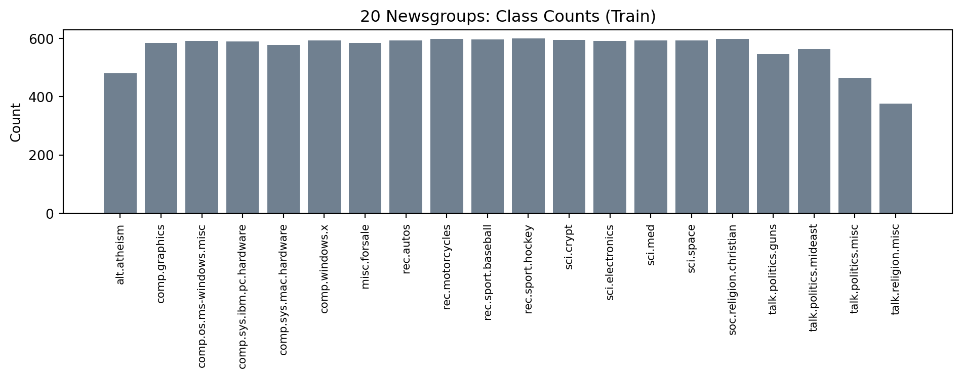

The “How”: Features and Modeling Choices

Key Takeaway: Sparse bag-of-words features remain strong baselines for topic classification, and regularization (L1 vs. L2) controls whether the model spreads weight broadly or focuses on a small set of salient features.

Bigram Intuition (Why add 2-grams?)

Bigrams capture short phrases that unigrams miss, such as “space shuttle”, “power supply”, or “real estate”. These phrases can be discriminative for certain topics.

from sklearn.feature_extraction.text import CountVectorizer

example_text = train_texts[0]
bigram_vec = CountVectorizer(stop_words="english", ngram_range=(2, 2), max_features=12)
bigram_vec.fit([example_text])
print("Example bigrams:", bigram_vec.get_feature_names_out())

Example bigrams: ['60s early' 'info funky' 'know tellme' 'late 60s' 'looked late'
 'looking car' 'model engine' 'production car' 'really small' 'saw day'
 'separate rest' 'small addition']

Model A: TF-IDF Unigrams + L2 Logistic Regression

TF-IDF reduces the weight of very common terms.
L2 regularization discourages large weights without forcing sparsity.

from sklearn.pipeline import Pipeline
from sklearn.feature_extraction.text import TfidfVectorizer
from sklearn.linear_model import LogisticRegression

model_a = Pipeline(
    [
        ("tfidf", TfidfVectorizer(stop_words="english", max_features=5000)),
        ("logreg", LogisticRegression(solver="lbfgs", penalty="l2", C=1.0, max_iter=1000)),
    ]
)
model_a.fit(train_texts, y_train)
pred_a = model_a.predict(test_texts)

/usr/local/anaconda3/envs/course-dev/lib/python3.13/site-packages/sklearn/linear_model/_logistic.py:1135: FutureWarning: 'penalty' was deprecated in version 1.8 and will be removed in 1.10. To avoid this warning, leave 'penalty' set to its default value and use 'l1_ratio' or 'C' instead. Use l1_ratio=0 instead of penalty='l2', l1_ratio=1 instead of penalty='l1', and C=np.inf instead of penalty=None.
  warnings.warn(

Model B: TF-IDF Unigrams + Bigrams + L1 Logistic Regression

Bigrams add short-phrase context.
L1 regularization produces sparse weights (feature selection).

model_b = Pipeline(
    [
        (
            "tfidf",
            TfidfVectorizer(
                stop_words="english",
                ngram_range=(1, 2),
                max_features=20000,
                min_df=2,
            ),
        ),
        ("logreg", LogisticRegression(solver="saga", penalty="l1", C=0.5, max_iter=1000)),
    ]
)
model_b.fit(train_texts, y_train)
pred_b = model_b.predict(test_texts)

/usr/local/anaconda3/envs/course-dev/lib/python3.13/site-packages/sklearn/linear_model/_logistic.py:1135: FutureWarning: 'penalty' was deprecated in version 1.8 and will be removed in 1.10. To avoid this warning, leave 'penalty' set to its default value and use 'l1_ratio' or 'C' instead. Use l1_ratio=0 instead of penalty='l2', l1_ratio=1 instead of penalty='l1', and C=np.inf instead of penalty=None.
  warnings.warn(
/usr/local/anaconda3/envs/course-dev/lib/python3.13/site-packages/sklearn/linear_model/_logistic.py:1160: UserWarning: Inconsistent values: penalty=l1 with l1_ratio=0.0. penalty is deprecated. Please use l1_ratio only.
  warnings.warn(

Evaluation: Accuracy, Precision, Recall, F1

Key Takeaway: Accuracy summarizes overall performance, but macro metrics highlight how well the model treats minority classes.

from sklearn.metrics import accuracy_score, precision_recall_fscore_support

def summarize(y_true, y_pred, name):
    acc = accuracy_score(y_true, y_pred)
    micro = precision_recall_fscore_support(y_true, y_pred, average="micro")
    macro = precision_recall_fscore_support(y_true, y_pred, average="macro")
    print(f"{name}: acc={acc:.3f}")
    print(f"  micro: P={micro[0]:.3f} R={micro[1]:.3f} F1={micro[2]:.3f}")
    print(f"  macro: P={macro[0]:.3f} R={macro[1]:.3f} F1={macro[2]:.3f}")
    return acc, macro[2]

acc_a, f1_macro_a = summarize(y_test, pred_a, "Model A")
acc_b, f1_macro_b = summarize(y_test, pred_b, "Model B")

Model A: acc=0.648
  micro: P=0.648 R=0.648 F1=0.648
  macro: P=0.650 R=0.635 F1=0.636
Model B: acc=0.557
  micro: P=0.557 R=0.557 F1=0.557
  macro: P=0.619 R=0.546 F1=0.567

F_beta (Recall Emphasis)

When missing a class is costly, we can emphasize recall with \(F_\beta\).

from sklearn.metrics import fbeta_score

f2_a = fbeta_score(y_test, pred_a, beta=2, average="macro")
f2_b = fbeta_score(y_test, pred_b, beta=2, average="macro")
print(f"Model A F2: {f2_a:.3f}")
print(f"Model B F2: {f2_b:.3f}")

Model A F2: 0.634
Model B F2: 0.550

Confusion Matrix (Best Macro F1)

Key Takeaway: The confusion matrix shows which topics are most often confused (e.g., similar sports or politics groups).

from sklearn.metrics import ConfusionMatrixDisplay

best_pred = pred_a if f1_macro_a >= f1_macro_b else pred_b
best_name = "Model A" if f1_macro_a >= f1_macro_b else "Model B"

fig, ax = plt.subplots(figsize=(10, 8))
disp = ConfusionMatrixDisplay.from_predictions(
    y_test,
    best_pred,
    display_labels=target_names,
    cmap="Blues",
    values_format="d",
    ax=ax,
)
disp.ax_.set_title(f"20 Newsgroups: Confusion Matrix ({best_name})")
plt.setp(disp.ax_.get_xticklabels(), rotation=90, ha="center", fontsize=8)
plt.setp(disp.ax_.get_yticklabels(), fontsize=8)
plt.tight_layout()
plt.show()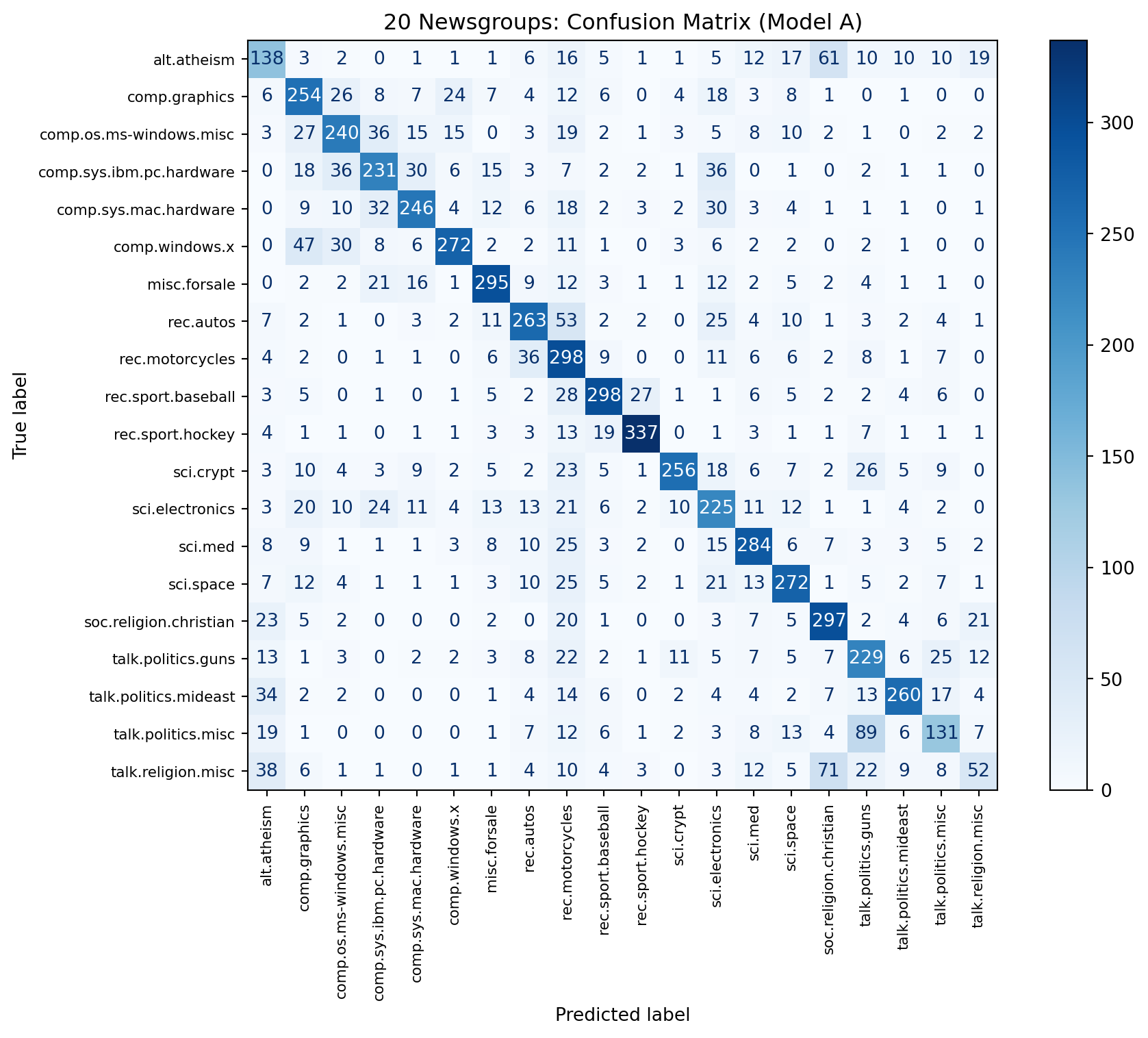

Bootstrapped Confidence Intervals

Key Takeaway: Bootstrapping quantifies uncertainty in accuracy and macro F1, giving a more honest comparison.

from sklearn.metrics import f1_score

def bootstrap_ci(y_true, y_pred, metric_fn, B=300, seed=11):
    rng = np.random.default_rng(seed)
    idx = np.arange(len(y_true))
    scores = np.empty(B)
    for i in range(B):
        sample = rng.choice(idx, size=len(idx), replace=True)
        scores[i] = metric_fn(y_true[sample], y_pred[sample])
    lo, hi = np.percentile(scores, [2.5, 97.5])
    return scores.mean(), lo, hi

acc_a_mean, acc_a_lo, acc_a_hi = bootstrap_ci(y_test, pred_a, accuracy_score)
acc_b_mean, acc_b_lo, acc_b_hi = bootstrap_ci(y_test, pred_b, accuracy_score)
f1_a_mean, f1_a_lo, f1_a_hi = bootstrap_ci(
    y_test, pred_a, lambda yt, yp: f1_score(yt, yp, average="macro")
)
f1_b_mean, f1_b_lo, f1_b_hi = bootstrap_ci(
    y_test, pred_b, lambda yt, yp: f1_score(yt, yp, average="macro")
)

labels = ["Accuracy", "Macro F1"]
x = np.arange(len(labels))
plt.figure(figsize=(7, 4))
plt.errorbar(
    x - 0.1,
    [acc_a_mean, f1_a_mean],
    yerr=[
        [acc_a_mean - acc_a_lo, f1_a_mean - f1_a_lo],
        [acc_a_hi - acc_a_mean, f1_a_hi - f1_a_mean],
    ],
    fmt="o",
    capsize=3,
    label="Model A",
)
plt.errorbar(
    x + 0.1,
    [acc_b_mean, f1_b_mean],
    yerr=[
        [acc_b_mean - acc_b_lo, f1_b_mean - f1_b_lo],
        [acc_b_hi - acc_b_mean, f1_b_hi - f1_b_mean],
    ],
    fmt="o",
    capsize=3,
    label="Model B",
)
plt.xticks(x, labels)
plt.ylabel("Score")
plt.title("20 Newsgroups: Bootstrapped 95% CIs")
plt.legend(frameon=False)
plt.grid(axis="y", alpha=0.3)
plt.tight_layout()
plt.show()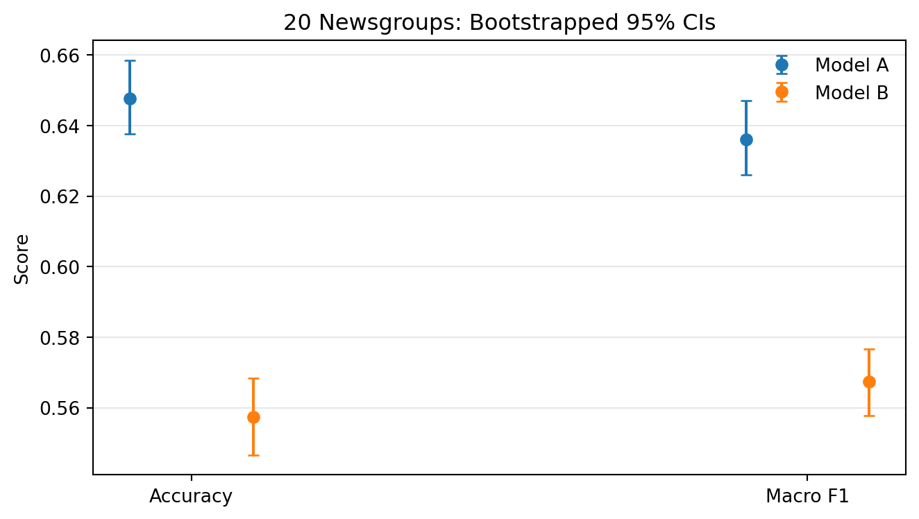

Model Comparison Takeaways

Model A (L2 + unigrams) tends to be stable and strong with fewer features.
Model B (L1 + uni+bi) can surface phrase-level cues but may overfit if feature limits are too high.
Macro metrics highlight whether minority topics are treated fairly.

Synthesis: Check Your Understanding

Why might macro F1 be more revealing than accuracy for this dataset?
What kinds of mistakes do you expect between closely related newsgroups (e.g., sports or politics)?
How would you adjust the pipeline if you cared most about recall for a specific topic?